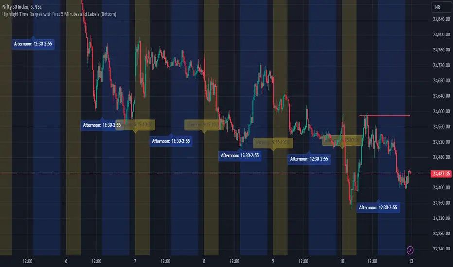
Volume-based Support & Resistance ZonesThe new and improved Support & Resistance Zones indicator is here. This indicator is based on high volume at fractal lows or fractal highs with the zones based on the size of the wick for that timeframe’s candle.
This helps traders visualize which price levels are of the most significance for either reversals or continuation of the trend when zones are broken and then re-tested.
Original script is thanks to synapticex and additional modifications is thanks to Lij_MC. Credit to both of them for most of the logic behind this script.
Since then I have made many changes to this script as noted below:
Changed default S/R lines from plots to lines, and gave option to user to change between solid line, dashed line, or dotted line for both S/R lines.
Added additional time frame and gave more TF options for TF1 other than current TF. Now you will have 4 time frames to plot S/R zones from.
Gave user option to easily change line thickness for all S/R lines.
Made it easier to change colors of S/R lines and zones by consolidating the options under settings (rather than under style).
Added extensions to active SR Zones to extend all the way right.
Added option to extend or not extend the previous S/R zones up to next S/R zone.
Added optional time frame labels to active S/R zones, with left and right options as well as option to adjust how far to the right label is set.
Fixed issue where the higher time frame S/R zone was not properly starting from the high/low of fractal. Now any higher time frame S/R will begin exactly at the High/Low points. Note that this may not work perfectly on stocks and if a fractal high/low is too many bars in the past, it will revert to a default max bars back to avoid script errors.
Added to script a function that will prevent S/R zones from lower time frames displaying while on a higher time frame. This helps clean up the chart quite a bit.
Created arrays for each time frame's boxes and lines so that the number of S/R zones can be controlled for each time frame and limit memory consumption.
New alert options added and customized alert messages.
- The way this indicator works is it looks for fractal highs or fractal lows with volume that pierces above the volume's Moving Average. This moving average value can be modified in the settings for each time frame.
- The fractal highs will be confirmed with 3 successive higher highs followed by 2 successive lower highs and vice versa for the fractal lows.
- The zone is created from the fractal high/low and the close of the candle for whatever time frame you selected. The bigger the zone, the more significant that zone is.
- You can disable any zone, change the zones to show lines only, and modify all the colors, transparencies, and thickness of lines for all the zones.
- To create alerts, you first want to enable the types of alerts you want for each time frame in the indicator's settings. Then after you apply changes, right click on one of the zones on the chart, and click "Add Alert on Vol S/R Zones". You do not need to add a title as the correct alert messages are already built-in.
- More changes will be coming in the future!
I hope you find this indicator useful, if so please give it a thumbs up!
If you have any suggestions or features you would like to see, just let me know in the comment section. Thanks and enjoy!
חפש סקריפטים עבור "high low"
lib_Indicators_v2_DTULibrary "lib_Indicators_v2_DTU"
This library functions returns included Moving averages, indicators with factorization, functions candles, function heikinashi and more.
Created it to feed as backend of my indicator/strategy "Indicators & Combinations Framework Advanced v2 " that will be released ASAP.
This is replacement of my previous indicator (lib_indicators_DT)
I will add an indicator example which will use this indicator named as "lib_indicators_v2_DTU example" to help the usage of this library
Additionally library will be updated with more indicators in the future
NOTES:
Indicator functions returns only one series :-(
plotcandle function returns candle series
INDICATOR LIST:
hide = 'DONT DISPLAY', //Dont display & calculate the indicator. (For my framework usage)
alma = 'alma(src,len,offset=0.85,sigma=6)', //Arnaud Legoux Moving Average
ama = 'ama(src,len,fast=14,slow=100)', //Adjusted Moving Average
acdst = 'accdist()', //Accumulation/distribution index.
cma = 'cma(src,len)', //Corrective Moving average
dema = 'dema(src,len)', //Double EMA (Same as EMA with 2 factor)
ema = 'ema(src,len)', //Exponential Moving Average
gmma = 'gmma(src,len)', //Geometric Mean Moving Average
hghst = 'highest(src,len)', //Highest value for a given number of bars back.
hl2ma = 'hl2ma(src,len)', //higest lowest moving average
hma = 'hma(src,len)', //Hull Moving Average.
lgAdt = 'lagAdapt(src,len,perclen=5,fperc=50)', //Ehler's Adaptive Laguerre filter
lgAdV = 'lagAdaptV(src,len,perclen=5,fperc=50)', //Ehler's Adaptive Laguerre filter variation
lguer = 'laguerre(src,len)', //Ehler's Laguerre filter
lsrcp = 'lesrcp(src,len)', //lowest exponential esrcpanding moving line
lexp = 'lexp(src,len)', //lowest exponential expanding moving line
linrg = 'linreg(src,len,loffset=1)', //Linear regression
lowst = 'lowest(src,len)', //Lovest value for a given number of bars back.
pcnl = 'percntl(src,len)', //percentile nearest rank. Calculates percentile using method of Nearest Rank.
pcnli = 'percntli(src,len)', //percentile linear interpolation. Calculates percentile using method of linear interpolation between the two nearest ranks.
rema = 'rema(src,len)', //Range EMA (REMA)
rma = 'rma(src,len)', //Moving average used in RSI. It is the exponentially weighted moving average with alpha = 1 / length.
sma = 'sma(src,len)', //Smoothed Moving Average
smma = 'smma(src,len)', //Smoothed Moving Average
supr2 = 'super2(src,len)', //Ehler's super smoother, 2 pole
supr3 = 'super3(src,len)', //Ehler's super smoother, 3 pole
strnd = 'supertrend(src,len,period=3)', //Supertrend indicator
swma = 'swma(src,len)', //Sine-Weighted Moving Average
tema = 'tema(src,len)', //Triple EMA (Same as EMA with 3 factor)
tma = 'tma(src,len)', //Triangular Moving Average
vida = 'vida(src,len)', //Variable Index Dynamic Average
vwma = 'vwma(src,len)', //Volume Weigted Moving Average
wma = 'wma(src,len)', //Weigted Moving Average
angle = 'angle(src,len)', //angle of the series (Use its Input as another indicator output)
atr = 'atr(src,len)', //average true range. RMA of true range.
bbr = 'bbr(src,len,mult=1)', //bollinger %%
bbw = 'bbw(src,len,mult=2)', //Bollinger Bands Width. The Bollinger Band Width is the difference between the upper and the lower Bollinger Bands divided by the middle band.
cci = 'cci(src,len)', //commodity channel index
cctbb = 'cctbbo(src,len)', //CCT Bollinger Band Oscilator
chng = 'change(src,len)', //Difference between current value and previous, source - source .
cmo = 'cmo(src,len)', //Chande Momentum Oscillator. Calculates the difference between the sum of recent gains and the sum of recent losses and then divides the result by the sum of all price movement over the same period.
cog = 'cog(src,len)', //The cog (center of gravity) is an indicator based on statistics and the Fibonacci golden ratio.
cpcrv = 'copcurve(src,len)', //Coppock Curve. was originally developed by Edwin "Sedge" Coppock (Barron's Magazine, October 1962).
corrl = 'correl(src,len)', //Correlation coefficient. Describes the degree to which two series tend to deviate from their ta.sma values.
count = 'count(src,len)', //green avg - red avg
dev = 'dev(src,len)', //ta.dev() Measure of difference between the series and it's ta.sma
fall = 'falling(src,len)', //ta.falling() Test if the `source` series is now falling for `length` bars long. (Use its Input as another indicator output)
kcr = 'kcr(src,len,mult=2)', //Keltner Channels Range
kcw = 'kcw(src,len,mult=2)', //ta.kcw(). Keltner Channels Width. The Keltner Channels Width is the difference between the upper and the lower Keltner Channels divided by the middle channel.
macd = 'macd(src,len)', //macd
mfi = 'mfi(src,len)', //Money Flow Index
nvi = 'nvi()', //Negative Volume Index
obv = 'obv()', //On Balance Volume
pvi = 'pvi()', //Positive Volume Index
pvt = 'pvt()', //Price Volume Trend
rise = 'rising(src,len)', //ta.rising() Test if the `source` series is now rising for `length` bars long. (Use its Input as another indicator output)
roc = 'roc(src,len)', //Rate of Change
rsi = 'rsi(src,len)', //Relative strength Index
smosc = 'smi_osc(src,len,fast=5, slow=34)', //smi Oscillator
smsig = 'smi_sig(src,len,fast=5, slow=34)', //smi Signal
stdev = 'stdev(src,len)', //Standart deviation
trix = 'trix(src,len)' , //the rate of change of a triple exponentially smoothed moving average.
tsi = 'tsi(src,len)', //True Strength Index
vari = 'variance(src,len)', //ta.variance(). Variance is the expectation of the squared deviation of a series from its mean (ta.sma), and it informally measures how far a set of numbers are spread out from their mean.
wilpc = 'willprc(src,len)', //Williams %R
wad = 'wad()', //Williams Accumulation/Distribution.
wvad = 'wvad()' //Williams Variable Accumulation/Distribution.
}
f_func(string, float, simple, float, float, float, simple) f_func Return selected indicator value with different parameters. New version. Use extra parameters for available indicators
Parameters:
string : FuncType_ indicator from the indicator list
float : src_ close, open, high, low,hl2, hlc3, ohlc4 or any
simple : int length_ indicator length
float : p1 extra parameter-1. active on Version 2 for defining multi arguments indicator input value. ex: lagAdapt(src_, length_,LAPercLen_=p1,FPerc_=p2)
float : p2 extra parameter-2. active on Version 2 for defining multi arguments indicator input value. ex: lagAdapt(src_, length_,LAPercLen_=p1,FPerc_=p2)
float : p3 extra parameter-3. active on Version 2 for defining multi arguments indicator input value. ex: lagAdapt(src_, length_,LAPercLen_=p1,FPerc_=p2)
simple : int version_ indicator version for backward compatibility. V1:dont use extra parameters p1,p2,p3 and use default values. V2: use extra parameters for available indicators
Returns: float Return calculated indicator value
fn_heikin(float, float, float, float) fn_heikin Return given src data (open, high,low,close) as heikin ashi candle values
Parameters:
float : o_ open value
float : h_ high value
float : l_ low value
float : c_ close value
Returns: float heikin ashi open, high,low,close vlues that will be used with plotcandle
fn_plotFunction(float, string, simple, bool) fn_plotFunction Return input src data with different plotting options
Parameters:
float : src_ indicator src_data or any other series.....
string : plotingType Ploting type of the function on the screen
simple : int stochlen_ length for plotingType for stochastic and PercentRank options
bool : plotSWMA Use SWMA for smoothing Ploting
Returns: float
fn_funcPlotV2(string, float, simple, float, float, float, simple, string, simple, bool, bool) fn_funcPlotV2 Return selected indicator value with different parameters. New version. Use extra parameters fora available indicators
Parameters:
string : FuncType_ indicator from the indicator list
float : src_data_ close, open, high, low,hl2, hlc3, ohlc4 or any
simple : int length_ indicator length
float : p1 extra parameter-1. active on Version 2 for defining multi arguments indicator input value. ex: lagAdapt(src_, length_,LAPercLen_=p1,FPerc_=p2)
float : p2 extra parameter-2. active on Version 2 for defining multi arguments indicator input value. ex: lagAdapt(src_, length_,LAPercLen_=p1,FPerc_=p2)
float : p3 extra parameter-3. active on Version 2 for defining multi arguments indicator input value. ex: lagAdapt(src_, length_,LAPercLen_=p1,FPerc_=p2)
simple : int version_ indicator version for backward compatibility. V1:dont use extra parameters p1,p2,p3 and use default values. V2: use extra parameters for available indicators
string : plotingType Ploting type of the function on the screen
simple : int stochlen_ length for plotingType for stochastic and PercentRank options
bool : plotSWMA Use SWMA for smoothing Ploting
bool : log_ Use log on function entries
Returns: float Return calculated indicator value
fn_factor(string, float, simple, float, float, float, simple, simple, string, simple, bool, bool) fn_factor Return selected indicator's factorization with given arguments
Parameters:
string : FuncType_ indicator from the indicator list
float : src_data_ close, open, high, low,hl2, hlc3, ohlc4 or any
simple : int length_ indicator length
float : p1 parameter-1. active on Version 2 for defining multi arguments indicator input value. ex: lagAdapt(src_, length_,LAPercLen_=p1,FPerc_=p2)
float : p2 parameter-2. active on Version 2 for defining multi arguments indicator input value. ex: lagAdapt(src_, length_,LAPercLen_=p1,FPerc_=p2)
float : p3 parameter-3. active on Version 2 for defining multi arguments indicator input value. ex: lagAdapt(src_, length_,LAPercLen_=p1,FPerc_=p2)
simple : int version_ indicator version for backward compatibility. V1:dont use extra parameters p1,p2,p3 and use default values. V2: use extra parameters for available indicators
simple : int fact_ Add double triple, Quatr factor to selected indicator (like converting EMA to 2-DEMA, 3-TEMA, 4-QEMA...)
string : plotingType Ploting type of the function on the screen
simple : int stochlen_ length for plotingType for stochastic and PercentRank options
bool : plotSWMA Use SWMA for smoothing Ploting
bool : log_ Use log on function entries
Returns: float Return result of the function
fn_plotCandles(string, simple, float, float, float, simple, string, simple, bool, bool, bool) fn_plotCandles Return selected indicator's candle values with different parameters also heikinashi is available
Parameters:
string : FuncType_ indicator from the indicator list
simple : int length_ indicator length
float : p1 parameter-1. active on Version 2 for defining multi arguments indicator input value. ex: lagAdapt(src_, length_,LAPercLen_=p1,FPerc_=p2)
float : p2 parameter-2. active on Version 2 for defining multi arguments indicator input value. ex: lagAdapt(src_, length_,LAPercLen_=p1,FPerc_=p2)
float : p3 parameter-3. active on Version 2 for defining multi arguments indicator input value. ex: lagAdapt(src_, length_,LAPercLen_=p1,FPerc_=p2)
simple : int version_ indicator version for backward compatibility. V1:dont use extra parameters p1,p2,p3 and use default values. V2: use extra parameters for available indicators
string : plotingType Ploting type of the function on the screen
simple : int stochlen_ length for plotingType for stochastic and PercentRank options
bool : plotSWMA Use SWMA for smoothing Ploting
bool : log_ Use log on function entries
bool : plotheikin_ Use Heikin Ashi on Plot
Returns: float
[MF] Auto Fibonacci LevelsDescription:
Automatically draw Fibonacci Pivot levels based on the previous (day's, week's or month's)
Range ( High-Low ). The HLC3 is used as the default Pivot level.
Unlike the "Auto Fibonacci Levels", this variation does not update
Levels on current day even if the price goes past the R3/S3 levels.
Timeframes: 1D, 1W, 1M
Range = (High - Low) - From previous Day, Week or month.
FIB LEVELS:
- Yellow = Pivot and Pivot Zone (HLC3 by default)
- red = R1,S1 Levels 0.236 * Range
- Green = R2,S2 Levels 0.368 * Range
- Lime = R3,S3 Levels 0.618 * Range
- Blue = R4,S4 Levels 0.786 * Range
- Gray = R5,S5 Levels 1.000 * Range
- Lime = R6,S6 Levels 1.236 * Range
- Red = R7,S7 Levels 1.382 * Range
- Blue = R8,S8 Levels 1.618 * Range
- Green = R9,S9 Levels 2.000 * Range
CLASSIC LEVELS:
- Yellow = Pivot and Pivot Zone (HLC3)
- Green = R1,S1 Levels (Pivot*2 - Low), (Pivot*2 - High)
- Lime = R2,S2 Levels ( Pivot + Range), ( Pivot - Range)
- Lime = R3,S3 Levels (High + 2*( Pivot - Low)), (Low - 2*(High - Pivot ))
- Blue = R4,S4 Levels (High + 3*( Pivot - Low)), (Low - 3*(High - Pivot ))
Refrences:
- Auto Daily Fib Levels R3.0 by JustUncleL
- Auto Fib by TheYangGuizi
- Monthly Dynamic Range Levels (Fibonaci) V0 by RicardoSantos
Modifications:
- Added next FIB Levels. (changes during the current cycle)
- Added FIB 0.236 Levels
- Added Option to change the colors of the Fib Levels
- Changed Default colors to the colors of Tradingview
- Upgraded to Version4 Pinescript
supertrendHere is an extensive library on different variations of supertrend.
Library "supertrend"
supertrend : Library dedicated to different variations of supertrend
supertrend_atr(length, multiplier, atrMaType, source, highSource, lowSource, waitForClose, delayed) supertrend_atr: Simple supertrend based on atr but also takes into consideration of custom MA Type, sources
Parameters:
length : : ATR Length
multiplier : : ATR Multiplier
atrMaType : : Moving Average type for ATR calculation. This can be sma, ema, hma, rma, wma, vwma, swma
source : : Default is close. Can Chose custom source
highSource : : Default is high. Can also use close price for both high and low source
lowSource : : Default is low. Can also use close price for both high and low source
waitForClose : : Considers source for direction change crossover if checked. Else, uses highSource and lowSource.
delayed : : if set to true lags supertrend atr stop based on target levels.
Returns: dir : Supertrend direction
supertrend : BuyStop if direction is 1 else SellStop
supertrend_bands(bandType, maType, length, multiplier, source, highSource, lowSource, waitForClose, useTrueRange, useAlternateSource, alternateSource, sticky) supertrend_bands: Simple supertrend based on atr but also takes into consideration of custom MA Type, sources
Parameters:
bandType : : Type of band used - can be bb, kc or dc
maType : : Moving Average type for Bands. This can be sma, ema, hma, rma, wma, vwma, swma
length : : Band Length
multiplier : : Std deviation or ATR multiplier for Bollinger Bands and Keltner Channel
source : : Default is close. Can Chose custom source
highSource : : Default is high. Can also use close price for both high and low source
lowSource : : Default is low. Can also use close price for both high and low source
waitForClose : : Considers source for direction change crossover if checked. Else, uses highSource and lowSource.
useTrueRange : : Used for Keltner channel. If set to false, then high-low is used as range instead of true range
useAlternateSource : - Custom source is used for Donchian Chanbel only if useAlternateSource is set to true
alternateSource : - Custom source for Donchian channel
sticky : : if set to true borders change only when price is beyond borders.
Returns: dir : Supertrend direction
supertrend : BuyStop if direction is 1 else SellStop
supertrend_zigzag(length, history, useAlternateSource, alternateSource, source, highSource, lowSource, waitForClose, atrlength, multiplier, atrMaType) supertrend_zigzag: Zigzag pivot based supertrend
Parameters:
length : : Zigzag Length
history : : number of historical pivots to consider
useAlternateSource : - Custom source is used for Zigzag only if useAlternateSource is set to true
alternateSource : - Custom source for Zigzag
source : : Default is close. Can Chose custom source
highSource : : Default is high. Can also use close price for both high and low source
lowSource : : Default is low. Can also use close price for both high and low source
waitForClose : : Considers source for direction change crossover if checked. Else, uses highSource and lowSource.
atrlength : : ATR Length
multiplier : : ATR Multiplier
atrMaType : : Moving Average type for ATR calculation. This can be sma, ema, hma, rma, wma, vwma, swma
Returns: dir : Supertrend direction
supertrend : BuyStop if direction is 1 else SellStop
taLibrary "ta"
█ OVERVIEW
This library holds technical analysis functions calculating values for which no Pine built-in exists.
Look first. Then leap.
█ FUNCTIONS
cagr(entryTime, entryPrice, exitTime, exitPrice)
It calculates the "Compound Annual Growth Rate" between two points in time. The CAGR is a notional, annualized growth rate that assumes all profits are reinvested. It only takes into account the prices of the two end points — not drawdowns, so it does not calculate risk. It can be used as a yardstick to compare the performance of two instruments. Because it annualizes values, the function requires a minimum of one day between the two end points (annualizing returns over smaller periods of times doesn't produce very meaningful figures).
Parameters:
entryTime : The starting timestamp.
entryPrice : The starting point's price.
exitTime : The ending timestamp.
exitPrice : The ending point's price.
Returns: CAGR in % (50 is 50%). Returns `na` if there is not >=1D between `entryTime` and `exitTime`, or until the two time points have not been reached by the script.
█ v2, Mar. 8, 2022
Added functions `allTimeHigh()` and `allTimeLow()` to find the highest or lowest value of a source from the first historical bar to the current bar. These functions will not look ahead; they will only return new highs/lows on the bar where they occur.
allTimeHigh(src)
Tracks the highest value of `src` from the first historical bar to the current bar.
Parameters:
src : (series int/float) Series to track. Optional. The default is `high`.
Returns: (float) The highest value tracked.
allTimeLow(src)
Tracks the lowest value of `src` from the first historical bar to the current bar.
Parameters:
src : (series int/float) Series to track. Optional. The default is `low`.
Returns: (float) The lowest value tracked.
█ v3, Sept. 27, 2022
This version includes the following new functions:
aroon(length)
Calculates the values of the Aroon indicator.
Parameters:
length (simple int) : (simple int) Number of bars (length).
Returns: ( [float, float ]) A tuple of the Aroon-Up and Aroon-Down values.
coppock(source, longLength, shortLength, smoothLength)
Calculates the value of the Coppock Curve indicator.
Parameters:
source (float) : (series int/float) Series of values to process.
longLength (simple int) : (simple int) Number of bars for the fast ROC value (length).
shortLength (simple int) : (simple int) Number of bars for the slow ROC value (length).
smoothLength (simple int) : (simple int) Number of bars for the weigted moving average value (length).
Returns: (float) The oscillator value.
dema(source, length)
Calculates the value of the Double Exponential Moving Average (DEMA).
Parameters:
source (float) : (series int/float) Series of values to process.
length (simple int) : (simple int) Length for the smoothing parameter calculation.
Returns: (float) The double exponentially weighted moving average of the `source`.
dema2(src, length)
An alternate Double Exponential Moving Average (Dema) function to `dema()`, which allows a "series float" length argument.
Parameters:
src : (series int/float) Series of values to process.
length : (series int/float) Length for the smoothing parameter calculation.
Returns: (float) The double exponentially weighted moving average of the `src`.
dm(length)
Calculates the value of the "Demarker" indicator.
Parameters:
length (simple int) : (simple int) Number of bars (length).
Returns: (float) The oscillator value.
donchian(length)
Calculates the values of a Donchian Channel using `high` and `low` over a given `length`.
Parameters:
length (int) : (series int) Number of bars (length).
Returns: ( [float, float, float ]) A tuple containing the channel high, low, and median, respectively.
ema2(src, length)
An alternate ema function to the `ta.ema()` built-in, which allows a "series float" length argument.
Parameters:
src : (series int/float) Series of values to process.
length : (series int/float) Number of bars (length).
Returns: (float) The exponentially weighted moving average of the `src`.
eom(length, div)
Calculates the value of the Ease of Movement indicator.
Parameters:
length (simple int) : (simple int) Number of bars (length).
div (simple int) : (simple int) Divisor used for normalzing values. Optional. The default is 10000.
Returns: (float) The oscillator value.
frama(source, length)
The Fractal Adaptive Moving Average (FRAMA), developed by John Ehlers, is an adaptive moving average that dynamically adjusts its lookback period based on fractal geometry.
Parameters:
source (float) : (series int/float) Series of values to process.
length (int) : (series int) Number of bars (length).
Returns: (float) The fractal adaptive moving average of the `source`.
ft(source, length)
Calculates the value of the Fisher Transform indicator.
Parameters:
source (float) : (series int/float) Series of values to process.
length (simple int) : (simple int) Number of bars (length).
Returns: (float) The oscillator value.
ht(source)
Calculates the value of the Hilbert Transform indicator.
Parameters:
source (float) : (series int/float) Series of values to process.
Returns: (float) The oscillator value.
ichimoku(conLength, baseLength, senkouLength)
Calculates values of the Ichimoku Cloud indicator, including tenkan, kijun, senkouSpan1, senkouSpan2, and chikou. NOTE: offsets forward or backward can be done using the `offset` argument in `plot()`.
Parameters:
conLength (int) : (series int) Length for the Conversion Line (Tenkan). The default is 9 periods, which returns the mid-point of the 9 period Donchian Channel.
baseLength (int) : (series int) Length for the Base Line (Kijun-sen). The default is 26 periods, which returns the mid-point of the 26 period Donchian Channel.
senkouLength (int) : (series int) Length for the Senkou Span 2 (Leading Span B). The default is 52 periods, which returns the mid-point of the 52 period Donchian Channel.
Returns: ( [float, float, float, float, float ]) A tuple of the Tenkan, Kijun, Senkou Span 1, Senkou Span 2, and Chikou Span values. NOTE: by default, the senkouSpan1 and senkouSpan2 should be plotted 26 periods in the future, and the Chikou Span plotted 26 days in the past.
ift(source)
Calculates the value of the Inverse Fisher Transform indicator.
Parameters:
source (float) : (series int/float) Series of values to process.
Returns: (float) The oscillator value.
kvo(fastLen, slowLen, trigLen)
Calculates the values of the Klinger Volume Oscillator.
Parameters:
fastLen (simple int) : (simple int) Length for the fast moving average smoothing parameter calculation.
slowLen (simple int) : (simple int) Length for the slow moving average smoothing parameter calculation.
trigLen (simple int) : (simple int) Length for the trigger moving average smoothing parameter calculation.
Returns: ( [float, float ]) A tuple of the KVO value, and the trigger value.
pzo(length)
Calculates the value of the Price Zone Oscillator.
Parameters:
length (simple int) : (simple int) Length for the smoothing parameter calculation.
Returns: (float) The oscillator value.
rms(source, length)
Calculates the Root Mean Square of the `source` over the `length`.
Parameters:
source (float) : (series int/float) Series of values to process.
length (int) : (series int) Number of bars (length).
Returns: (float) The RMS value.
rwi(length)
Calculates the values of the Random Walk Index.
Parameters:
length (simple int) : (simple int) Lookback and ATR smoothing parameter length.
Returns: ( [float, float ]) A tuple of the `rwiHigh` and `rwiLow` values.
stc(source, fast, slow, cycle, d1, d2)
Calculates the value of the Schaff Trend Cycle indicator.
Parameters:
source (float) : (series int/float) Series of values to process.
fast (simple int) : (simple int) Length for the MACD fast smoothing parameter calculation.
slow (simple int) : (simple int) Length for the MACD slow smoothing parameter calculation.
cycle (simple int) : (simple int) Number of bars for the Stochastic values (length).
d1 (simple int) : (simple int) Length for the initial %D smoothing parameter calculation.
d2 (simple int) : (simple int) Length for the final %D smoothing parameter calculation.
Returns: (float) The oscillator value.
stochFull(periodK, smoothK, periodD)
Calculates the %K and %D values of the Full Stochastic indicator.
Parameters:
periodK (simple int) : (simple int) Number of bars for Stochastic calculation. (length).
smoothK (simple int) : (simple int) Number of bars for smoothing of the %K value (length).
periodD (simple int) : (simple int) Number of bars for smoothing of the %D value (length).
Returns: ( [float, float ]) A tuple of the slow %K and the %D moving average values.
stochRsi(lengthRsi, periodK, smoothK, periodD, source)
Calculates the %K and %D values of the Stochastic RSI indicator.
Parameters:
lengthRsi (simple int) : (simple int) Length for the RSI smoothing parameter calculation.
periodK (simple int) : (simple int) Number of bars for Stochastic calculation. (length).
smoothK (simple int) : (simple int) Number of bars for smoothing of the %K value (length).
periodD (simple int) : (simple int) Number of bars for smoothing of the %D value (length).
source (float) : (series int/float) Series of values to process. Optional. The default is `close`.
Returns: ( [float, float ]) A tuple of the slow %K and the %D moving average values.
supertrend(factor, atrLength, wicks)
Calculates the values of the SuperTrend indicator with the ability to take candle wicks into account, rather than only the closing price.
Parameters:
factor (float) : (series int/float) Multiplier for the ATR value.
atrLength (simple int) : (simple int) Length for the ATR smoothing parameter calculation.
wicks (simple bool) : (simple bool) Condition to determine whether to take candle wicks into account when reversing trend, or to use the close price. Optional. Default is false.
Returns: ( [float, int ]) A tuple of the superTrend value and trend direction.
szo(source, length)
Calculates the value of the Sentiment Zone Oscillator.
Parameters:
source (float) : (series int/float) Series of values to process.
length (simple int) : (simple int) Length for the smoothing parameter calculation.
Returns: (float) The oscillator value.
t3(source, length, vf)
Calculates the value of the Tilson Moving Average (T3).
Parameters:
source (float) : (series int/float) Series of values to process.
length (simple int) : (simple int) Length for the smoothing parameter calculation.
vf (simple float) : (simple float) Volume factor. Affects the responsiveness.
Returns: (float) The Tilson moving average of the `source`.
t3Alt(source, length, vf)
An alternate Tilson Moving Average (T3) function to `t3()`, which allows a "series float" `length` argument.
Parameters:
source (float) : (series int/float) Series of values to process.
length (float) : (series int/float) Length for the smoothing parameter calculation.
vf (simple float) : (simple float) Volume factor. Affects the responsiveness.
Returns: (float) The Tilson moving average of the `source`.
tema(source, length)
Calculates the value of the Triple Exponential Moving Average (TEMA).
Parameters:
source (float) : (series int/float) Series of values to process.
length (simple int) : (simple int) Length for the smoothing parameter calculation.
Returns: (float) The triple exponentially weighted moving average of the `source`.
tema2(source, length)
An alternate Triple Exponential Moving Average (TEMA) function to `tema()`, which allows a "series float" `length` argument.
Parameters:
source (float) : (series int/float) Series of values to process.
length (float) : (series int/float) Length for the smoothing parameter calculation.
Returns: (float) The triple exponentially weighted moving average of the `source`.
trima(source, length)
Calculates the value of the Triangular Moving Average (TRIMA).
Parameters:
source (float) : (series int/float) Series of values to process.
length (int) : (series int) Number of bars (length).
Returns: (float) The triangular moving average of the `source`.
trima2(src, length)
An alternate Triangular Moving Average (TRIMA) function to `trima()`, which allows a "series int" length argument.
Parameters:
src : (series int/float) Series of values to process.
length : (series int) Number of bars (length).
Returns: (float) The triangular moving average of the `src`.
trix(source, length, signalLength, exponential)
Calculates the values of the TRIX indicator.
Parameters:
source (float) : (series int/float) Series of values to process.
length (simple int) : (simple int) Length for the smoothing parameter calculation.
signalLength (simple int) : (simple int) Length for smoothing the signal line.
exponential (simple bool) : (simple bool) Condition to determine whether exponential or simple smoothing is used. Optional. The default is `true` (exponential smoothing).
Returns: ( [float, float, float ]) A tuple of the TRIX value, the signal value, and the histogram.
uo(fastLen, midLen, slowLen)
Calculates the value of the Ultimate Oscillator.
Parameters:
fastLen (simple int) : (series int) Number of bars for the fast smoothing average (length).
midLen (simple int) : (series int) Number of bars for the middle smoothing average (length).
slowLen (simple int) : (series int) Number of bars for the slow smoothing average (length).
Returns: (float) The oscillator value.
vhf(source, length)
Calculates the value of the Vertical Horizontal Filter.
Parameters:
source (float) : (series int/float) Series of values to process.
length (simple int) : (simple int) Number of bars (length).
Returns: (float) The oscillator value.
vi(length)
Calculates the values of the Vortex Indicator.
Parameters:
length (simple int) : (simple int) Number of bars (length).
Returns: ( [float, float ]) A tuple of the viPlus and viMinus values.
vzo(length)
Calculates the value of the Volume Zone Oscillator.
Parameters:
length (simple int) : (simple int) Length for the smoothing parameter calculation.
Returns: (float) The oscillator value.
williamsFractal(period)
Detects Williams Fractals.
Parameters:
period (int) : (series int) Number of bars (length).
Returns: ( [bool, bool ]) A tuple of an up fractal and down fractal. Variables are true when detected.
wpo(length)
Calculates the value of the Wave Period Oscillator.
Parameters:
length (simple int) : (simple int) Length for the smoothing parameter calculation.
Returns: (float) The oscillator value.
█ v7, Nov. 2, 2023
This version includes the following new and updated functions:
atr2(length)
An alternate ATR function to the `ta.atr()` built-in, which allows a "series float" `length` argument.
Parameters:
length (float) : (series int/float) Length for the smoothing parameter calculation.
Returns: (float) The ATR value.
changePercent(newValue, oldValue)
Calculates the percentage difference between two distinct values.
Parameters:
newValue (float) : (series int/float) The current value.
oldValue (float) : (series int/float) The previous value.
Returns: (float) The percentage change from the `oldValue` to the `newValue`.
donchian(length)
Calculates the values of a Donchian Channel using `high` and `low` over a given `length`.
Parameters:
length (int) : (series int) Number of bars (length).
Returns: ( [float, float, float ]) A tuple containing the channel high, low, and median, respectively.
highestSince(cond, source)
Tracks the highest value of a series since the last occurrence of a condition.
Parameters:
cond (bool) : (series bool) A condition which, when `true`, resets the tracking of the highest `source`.
source (float) : (series int/float) Series of values to process. Optional. The default is `high`.
Returns: (float) The highest `source` value since the last time the `cond` was `true`.
lowestSince(cond, source)
Tracks the lowest value of a series since the last occurrence of a condition.
Parameters:
cond (bool) : (series bool) A condition which, when `true`, resets the tracking of the lowest `source`.
source (float) : (series int/float) Series of values to process. Optional. The default is `low`.
Returns: (float) The lowest `source` value since the last time the `cond` was `true`.
relativeVolume(length, anchorTimeframe, isCumulative, adjustRealtime)
Calculates the volume since the last change in the time value from the `anchorTimeframe`, the historical average volume using bars from past periods that have the same relative time offset as the current bar from the start of its period, and the ratio of these volumes. The volume values are cumulative by default, but can be adjusted to non-accumulated with the `isCumulative` parameter.
Parameters:
length (simple int) : (simple int) The number of periods to use for the historical average calculation.
anchorTimeframe (simple string) : (simple string) The anchor timeframe used in the calculation. Optional. Default is "D".
isCumulative (simple bool) : (simple bool) If `true`, the volume values will be accumulated since the start of the last `anchorTimeframe`. If `false`, values will be used without accumulation. Optional. The default is `true`.
adjustRealtime (simple bool) : (simple bool) If `true`, estimates the cumulative value on unclosed bars based on the data since the last `anchor` condition. Optional. The default is `false`.
Returns: ( [float, float, float ]) A tuple of three float values. The first element is the current volume. The second is the average of volumes at equivalent time offsets from past anchors over the specified number of periods. The third is the ratio of the current volume to the historical average volume.
rma2(source, length)
An alternate RMA function to the `ta.rma()` built-in, which allows a "series float" `length` argument.
Parameters:
source (float) : (series int/float) Series of values to process.
length (float) : (series int/float) Length for the smoothing parameter calculation.
Returns: (float) The rolling moving average of the `source`.
supertrend2(factor, atrLength, wicks)
An alternate SuperTrend function to `supertrend()`, which allows a "series float" `atrLength` argument.
Parameters:
factor (float) : (series int/float) Multiplier for the ATR value.
atrLength (float) : (series int/float) Length for the ATR smoothing parameter calculation.
wicks (simple bool) : (simple bool) Condition to determine whether to take candle wicks into account when reversing trend, or to use the close price. Optional. Default is `false`.
Returns: ( [float, int ]) A tuple of the superTrend value and trend direction.
vStop(source, atrLength, atrFactor)
Calculates an ATR-based stop value that trails behind the `source`. Can serve as a possible stop-loss guide and trend identifier.
Parameters:
source (float) : (series int/float) Series of values that the stop trails behind.
atrLength (simple int) : (simple int) Length for the ATR smoothing parameter calculation.
atrFactor (float) : (series int/float) The multiplier of the ATR value. Affects the maximum distance between the stop and the `source` value. A value of 1 means the maximum distance is 100% of the ATR value. Optional. The default is 1.
Returns: ( [float, bool ]) A tuple of the volatility stop value and the trend direction as a "bool".
vStop2(source, atrLength, atrFactor)
An alternate Volatility Stop function to `vStop()`, which allows a "series float" `atrLength` argument.
Parameters:
source (float) : (series int/float) Series of values that the stop trails behind.
atrLength (float) : (series int/float) Length for the ATR smoothing parameter calculation.
atrFactor (float) : (series int/float) The multiplier of the ATR value. Affects the maximum distance between the stop and the `source` value. A value of 1 means the maximum distance is 100% of the ATR value. Optional. The default is 1.
Returns: ( [float, bool ]) A tuple of the volatility stop value and the trend direction as a "bool".
Removed Functions:
allTimeHigh(src)
Tracks the highest value of `src` from the first historical bar to the current bar.
allTimeLow(src)
Tracks the lowest value of `src` from the first historical bar to the current bar.
trima2(src, length)
An alternate Triangular Moving Average (TRIMA) function to `trima()`, which allows a
"series int" length argument.
My:HTF O/H/L/C█ MY Higher Time Frame Open / High / Low / Close
This indicator shows one line per Higher Time Frame Price of Interest.
We are interested to know whether we are currently seeing support or resistance at previous daily / weekly / monthly price of interest.
Each price of interest can be displayed or hidden in the configuration. Each line has a label attached to it with the (short) label on it to help identifying what is this line.
Price of interest with (short) label :
Current Daily Open (CDO)
Current Daily High (CDH)
Current Daily Low (CDL)
Previous Daily Open (PDO)
Previous Daily High (PDH)
Previous Daily Low (PDL)
Previous Daily Close (PDC)
Current Weekly Open (CWO)
Current Weekly High (CWH)
Current Weekly Low (CWL)
Previous Weekly Open (PWO)
Previous Weekly High (PWH)
Previous Weekly Low (PWL)
Previous Weekly Close (PWC)
Current Monthly Open (CMO)
Current Monthly High (CMH)
Current Monthly Low (CML)
Previous Monthly Open (PMO)
Previous Monthly High (PMH)
Previous Monthly Low (PML)
Previous Monthly Close (PMC)
Strat Assistant FTC OnlyStrat Assistant FTC Only
----------------------------
█ OVERVIEW
This script is intended to provide full time frame continuity information for almost all time frames (3, 5, 15, 30, 60, 4H, Day, Week, Month, Quarter)
When added, the script provides a visual indicator to the right at the current price level with indicators for the various time frames in terms of price action and candle type.
█ DETAIL
----------
Output
Time Frames: 3min, 5min, 15min, 30min, 60min, 4 Hour, Day, Week, Month Quarter
Time Frame Labels: 3, 5, 15, 30, 60, H, 4H, D, W, M, Q
Current Candle Time Frame Price Action: displayed below time frame labels. RED + Arrow Down (open > close) or GREEN + Arrow Up (open =< close)
Time Frame Compare: displayed above time frame labels. Current high/low vs prior high/low are compared. IN = Inside/Yellow (current high/low inside prior), O = Outside/Fuchsia (current high/low both greater and less than prior high/low), 2U = Up/Green (current high higher than prior, and low not lower), 2D = Down/Red (current lows lower than prior lows, and high not higher)
Will not show time frames lower than the one currently selected
Best Practices
----------
Had to decouple this from the other scripts because Trading View limits how much you can plot/show
May be a little slow at times, analyzing a lot of time periods/data be patient.
MA DerivativesMA Derivatives basicly using Ichimoku Cloud and some additional moving averages for traders.
A. ICHIMOKU
Tenkan-sen (Conversion Line): (9-period high + 9-period low)/2
On a daily chart , this line is the midpoint of the 9-day high-low range, which is almost two weeks.
Kijun-sen (Base Line): (26-period high + 26-period low)/2
On a daily chart , this line is the midpoint of the 26-day high-low range, which is almost one month.
Senkou Span A (Leading Span A): (Conversion Line + Base Line)/2
This is the midpoint between the Conversion Line and the Base Line. The Leading Span A forms one of the two Cloud boundaries. It is referred to as “Leading” because it is plotted 26 periods in the future and forms the faster Cloud boundary.
Senkou Span B (Leading Span B): (52-period high + 52-period low)/2
On the daily chart , this line is the midpoint of the 52-day high-low range, which is a little less than 3 months. The default calculation setting is 52 periods, but it can be adjusted. This value is plotted 26 periods in the future and forms the slower Cloud boundary.
Chikou Span: Represents the closing price and is plotted 26 days back.
Kumo Cloud: Kumo cloud between Senkuo Span A and Senkou Span B lines. It can be green or red. Color can be change with the trend.
You can use Ichimoku for buy&sell strategy
For Buying Strategy
- Tenkansen (Conversion Line) should crossover Kijunsen (Base line) above the highest line of cloud
- Price should be above the highest line of cloud
- Chikouspan should be above the cloud
For Selling Strategy
- Kijunsen (Base Line) should crossover Tenkansen (Conversion Line) below the lowest line of cloud
- Price should be below the lowest line of cloud
- Chikouspan should be below the cloud
B. SIMPLE MOVING AVERAGES
The indicator has some of Simple Moving Averages
It includes:
-Simple Moving Average 50
-Simple Moving Average 100
-Simple Moving Average 200
C. EXPONENTIAL MOVING AVERAGES
The indicator has some of Simple Moving Averages
It includes:
-Exponential Moving Average 9
-Exponential Moving Average 21
-Exponential Moving Average 50
D. BOLLINGER BAND
Bollinger Bands are a type of price envelope developed by John BollingerOpens in a new window. (Price envelopes define upper and lower price range levels.) Bollinger Bands are envelopes plotted at a standard deviation level above and below a simple moving average of the price. Because the distance of the bands is based on standard deviation, they adjust to volatility swings in the underlying price.
Bollinger Bands use 2 parameters, Period and Standard Deviations, StdDev. The default values are 20 for period, and 2 for standard deviations, although you may customize the combinations.
Bollinger bands help determine whether prices are high or low on a relative basis. They are used in pairs, both upper and lower bands and in conjunction with a moving average. Further, the pair of bands is not intended to be used on its own. Use the pair to confirm signals given with other indicators.
How this indicator works
When the bands tighten during a period of low volatility, it raises the likelihood of a sharp price move in either direction. This may begin a trending move. Watch out for a false move in opposite direction which reverses before the proper trend begins.
When the bands separate by an unusual large amount, volatility increases and any existing trend may be ending.
Prices have a tendency to bounce within the bands' envelope, touching one band then moving to the other band. You can use these swings to help identify potential profit targets. For example, if a price bounces off the lower band and then crosses above the moving average, the upper band then becomes the profit target.
Price can exceed or hug a band envelope for prolonged periods during strong trends. On divergence with a momentum oscillator, you may want to do additional research to determine if taking additional profits is appropriate for you.
A strong trend continuation can be expected when the price moves out of the bands. However, if prices move immediately back inside the band, then the suggested strength is negated.
Calculation
First, calculate a simple moving average. Next, calculate the standard deviation over the same number of periods as the simple moving average. For the upper band, add the standard deviation to the moving average. For the lower band, subtract the standard deviation from the moving average.
Typical values used:
Short term: 10 day moving average, bands at 1.5 standard deviations. (1.5 times the standard dev. +/- the SMA)
Medium term: 20 day moving average, bands at 2 standard deviations.
Long term: 50 day moving average, bands at 2.5 standard deviations.
E. ADJUSTABLE MOVING AVERAGES
And this script has also 2 adjustable moving average
- 1 Adjustable Simple Moving Average
- 1 Adjustable Exponential Moving Average
You can just change the length for using this tool.
HhLl-OscilatorSimple oscillator which checks how many highs and how many lows the price is making. Parameters are as explained below:
lookback - Checks how many highs and lows it is making in these many bars. Sum of all highs and lows are taken for plotting.
periods - Initial period to check high and lows
multiples - Number of multiples on initial period for which highs and lows are checked
colorCandles - CandleColor based on the oscillator
If periods is 20 and multiples is 5 and loopback is 10
Indicator checks for last 10 bars how many highs/lows are made for 20, 40, 60, 80 and 100 periods. Sum of all highs and lows are plotted on the oscillator overlay
Expanded Floor PivotsHello Everyone,
The Expanded Floor Pivots is introduced in the book "Secrets of a Pivot Boss: Revealing Proven Methods for Profiting in the Market " by Franklin Ochoa. He added four new levels: S4, R4, BC and TC. There are many great ideas in the book, such using these levels, following trend, time price opportunity and much more. (Thanks to @tonyjab for pushing me to read this book)
The definition/formula of the levels defined in the book:
r1 = 2 * pivot - Low
r2 = pivot + (High - Low)
r3 = r1 + (High - Low)
r4 = r3 + (r2 - r1)
tc = (pivot - bc) + pivot
pivot = (High + Low + Close) / 3
bc = (High + Low) / 2
s1 = 2 * pivot - High
s2 = pivot - (High - Low)
s3 = s1 - (High - Low)
s4 = s3 - (s1 - s2)
The area between TC and BC is used as Pivot Channel, (blue area in the chart). you can see how it helps on identifying the trend.
Options:
By default the script decides Higher Time Frame but if you want you can set HTF as you wish.
You can choose line style as: Solid, Circles or Cross
and also you have option to show only last period or all historical levels.
Enjoy!
Ease of Movement WatcherHere’s a handy Ease of Movement(EMV) Indicator. I tried to include detailed comments so that anyone that’s learning pine can follow along.
The Ease of Movement Indicator is a volume based oscillator that is designed to measure the ease (or movability) of price movement for a security. The EMV is a centered oscillator, meaning that values can fluctuate above and below zero.
To understand how to use and interpret the EMV Indicator, its crucial to first understand its two main calculations :
Distance Moved = ((high + low) / 2) - ((high + low ) / 2)
-This is the difference between the current period’s midpoint and the previous period’s
midpoint.
Box Ratio = (volume / 100,000) / (high - low)
-When calculating the Box Ratio, it is common to divide the volume by 100,000 for a clearer visualization of the data. However, users can choose
to modify this value with the ‘volumeDiv’ input.
The Ease of Movement Value is then pretty simple to calculate:
EMV = (Distance Moved / Box Ratio)
The indicator then plots a SMA of the previous 24 EMV Values.
Looking at the formula, we know that combining low volume with a large {high, low} range will result in a relatively small box ratio value. Thus, we know that the EMV value for that period will be higher since EMV is found by dividing the Distance Moved by the Box Ratio.
Here’s a simple guide to interpreting the EMV:
- If (EMV > 0)
then price is increasing with relative ease.
-If (EMV < 0)
then price is decreasing with relative ease.
- If high-low range is large and volume is low
then ease of movement is high.
-If high-low range is small and volume is high
then ease of movement is low.
The Chart:
-The histogram represents the Simple Moving Average of EMV Values. The default length is 24, but users can adjust this value at the inputs menu(I've
found 24 works best).
-The teal and pink dotted lines represent the standard deviation of the SMA of EMV values multiplied by 2.5.
-The histogram turns dark green when the EMV SMA is greater than the top teal dotted standard deviations line.
-The histogram turns maroon when the EMV SMA falls below the bottom pink standard deviation line.
How To Use:
Enter a long position when the most recent EMV SMA value was below the lower pink stand. dev. line and the current EMV SMA value rises above that
same pink line. That means the previous bar was maroon and the current bar is not.
If the user enables the option to show entry points, a green dot will be plotted when it is time to enter a long position.
Exit the long position when the most recent EMV SMA value was above the upper green standard deviation line and the current EMV SMA value falls
below that same line. If this is true, then the previous bar will be dark green, and the current will be light green.
If the ‘showExits’ option is enabled, then a red dot will be plotted when it is time to exit the long position.
Input Options:
- 'volumeDiv' : Integer. Used in the calculation of Box Ratio.
- 'lenSMA' : Integer. The length of the Simple Moving Average of Ease of Movement Values.
- 'showStDev' : Bool. If true, dotted green and red lines will be shown at values equal to 2.5 * standard deviation of emvSMA and -2.5 * standard deviation of
emvSMA.
- 'showEntries' and 'showExits' : Bool. If true, a green circle will be plotted at long entry points and a red circle will be plotted at long exit points.
- 'changeBgColor': Bool. If true, the background color will change to green when it is time to enter a long position and red when it is time to exit.
Alerts:
- When it is time to enter a long position, an alert with the message "EMV Tracker - Enter Long" is sent.
- When it is time to exit a long position, an alert with the message "EMV Tracker - Exit Long" is sent.
NOTE:
- I usually use this indicator to confirm signals from other indicators rather than relying on it solely.
- Most accurate signals are generated on 30 minutes with the default input values I've set in the script.
Shoot me a message if you have any ideas for modifications or questions.
~ Happy Trading ~
SpatialIndexYou can start using this now by inserthing this at the top of your indicator/strategy/library.
import ArunaReborn/SpatialIndex/1 as SI
Overview
SpatialIndex is a high-performance Pine Script library that implements price-bucketed spatial indexing for efficient proximity queries on large datasets. Instead of scanning through hundreds or thousands of items linearly (O(n)), this library provides O(k) bucket lookup where k is typically just a handful of buckets, dramatically improving performance for price-based filtering operations.
This library works with any data type through index-based references, making it universally applicable for support/resistance levels, pivot points, order zones, pattern detection points, Fair Value Gaps, and any other price-based data that needs frequent proximity queries.
Why This Library Exists
The Problem
When building advanced technical indicators that track large numbers of price levels (support/resistance zones, pivot points, order blocks, etc.), you often need to answer questions like:
- *"Which levels are within 5% of the current price?"*
- *"What zones overlap with this price range?"*
- *"Are there any significant levels near my entry point?"*
The naive approach is to loop through every single item and check its price. For 500 levels across multiple timeframes, this means 500 comparisons every bar . On instruments with thousands of historical bars, this quickly becomes a performance bottleneck that can cause scripts to time out or lag.
The Solution
SpatialIndex solves this by organizing items into price buckets —like filing cabinets organized by price range. When you query for items near $50,000, the library only looks in the relevant buckets (e.g., $49,000-$51,000 range), ignoring all other price regions entirely.
Performance Example:
- Linear scan: Check 500 items = 500 comparisons per query
- Spatial index: Check 3-5 buckets with ~10 items each = 30-50 comparisons per query
- Result: 10-16x faster queries
Key Features
Core Capabilities
- ✅ Generic Design : Works with any data type via index references
- ✅ Multiple Index Strategies : Fixed bucket size or ATR-based dynamic sizing
- ✅ Range Support : Index items that span price ranges (zones, gaps, channels)
- ✅ Efficient Queries : O(k) bucket lookup instead of O(n) linear scan
- ✅ Multiple Query Types : Proximity percentage, fixed range, exact price with tolerance
- ✅ Dynamic Updates : Add, remove, update items in O(1) time
- ✅ Batch Operations : Efficient bulk removal and reindexing
- ✅ Query Caching : Optional caching for repeated queries within same bar
- ✅ Statistics & Debugging : Built-in stats and diagnostic functions
### Advanced Features
- ATR-Based Bucketing : Automatically adjusts bucket sizes based on volatility
- Multi-Bucket Spanning : Items that span ranges are indexed in all overlapping buckets
- Reindexing Support : Handles array removals with automatic index shifting
- Cache Management : Configurable query caching with automatic invalidation
- Empty Bucket Cleanup : Automatically removes empty buckets to minimize memory
How It Works
The Bucketing Concept
Think of price space as divided into discrete buckets, like a histogram:
```
Price Range: $98-$100 $100-$102 $102-$104 $104-$106 $106-$108
Bucket Key: 49 50 51 52 53
Items:
```
When you query for items near $103:
1. Calculate which buckets overlap the $101.50-$104.50 range (keys 50, 51, 52)
2. Return items from only those buckets:
3. Never check items in buckets 49 or 53
Bucket Size Selection
Fixed Size Mode:
```pine
var SI.SpatialBucket index = SI.newSpatialBucket(2.0) // $2 per bucket
```
- Good for: Instruments with stable price ranges
- Example: For stocks trading at $100, 2.0 = 2% increments
ATR-Based Mode:
```pine
float atr = ta.atr(14)
var SI.SpatialBucket index = SI.newSpatialBucketATR(1.0, atr) // 1x ATR per bucket
SI.updateATR(index, atr) // Update each bar
```
- Good for: Instruments with varying volatility
- Adapts automatically to market conditions
- 1.0 multiplier = one bucket spans one ATR unit
Optimal Bucket Size:
The library includes a helper function to calculate optimal size:
```pine
float optimalSize = SI.calculateOptimalBucketSize(close, 5.0) // For 5% proximity queries
```
This ensures queries span approximately 3 buckets for optimal performance.
Index-Based Architecture
The library doesn't store your actual data—it only stores indices that point to your external arrays:
```pine
// Your data
var array levels = array.new()
var array types = array.new()
var array ages = array.new()
// Your index
var SI.SpatialBucket index = SI.newSpatialBucket(2.0)
// Add a level
array.push(levels, 50000.0)
array.push(types, "support")
array.push(ages, 0)
SI.add(index, array.size(levels) - 1, 50000.0) // Store index 0
// Query near current price
SI.QueryResult result = SI.queryProximity(index, close, 5.0)
for idx in result.indices
float level = array.get(levels, idx)
string type = array.get(types, idx)
// Work with your actual data
```
This design means:
- ✅ Works with any data structure you define
- ✅ No data duplication
- ✅ Minimal memory footprint
- ✅ Full control over your data
---
Usage Guide
Basic Setup
```pine
// Import library
import username/SpatialIndex/1 as SI
// Create index
var SI.SpatialBucket index = SI.newSpatialBucket(2.0)
// Your data arrays
var array supportLevels = array.new()
var array touchCounts = array.new()
```
Adding Items
Single Price Point:
```pine
// Add a support level at $50,000
array.push(supportLevels, 50000.0)
array.push(touchCounts, 1)
int levelIdx = array.size(supportLevels) - 1
SI.add(index, levelIdx, 50000.0)
```
Price Range (Zones/Gaps):
```pine
// Add a resistance zone from $51,000 to $52,000
array.push(zoneBottoms, 51000.0)
array.push(zoneTops, 52000.0)
int zoneIdx = array.size(zoneBottoms) - 1
SI.addRange(index, zoneIdx, 51000.0, 52000.0) // Indexed in all overlapping buckets
```
Querying Items
Proximity Query (Percentage):
```pine
// Find all levels within 5% of current price
SI.QueryResult result = SI.queryProximity(index, close, 5.0)
if array.size(result.indices) > 0
for idx in result.indices
float level = array.get(supportLevels, idx)
// Process nearby level
```
Fixed Range Query:
```pine
// Find all items between $49,000 and $51,000
SI.QueryResult result = SI.queryRange(index, 49000.0, 51000.0)
```
Exact Price with Tolerance:
```pine
// Find items at exactly $50,000 +/- $100
SI.QueryResult result = SI.queryAt(index, 50000.0, 100.0)
```
Removing Items
Safe Removal Pattern:
```pine
SI.QueryResult result = SI.queryProximity(index, close, 5.0)
if array.size(result.indices) > 0
// IMPORTANT: Sort descending to safely remove from arrays
array sorted = SI.sortIndicesDescending(result)
for idx in sorted
// Remove from index
SI.remove(index, idx)
// Remove from your data arrays
array.remove(supportLevels, idx)
array.remove(touchCounts, idx)
// Reindex to maintain consistency
SI.reindexAfterRemoval(index, idx)
```
Batch Removal (More Efficient):
```pine
// Collect indices to remove
array toRemove = array.new()
for i = 0 to array.size(supportLevels) - 1
if array.get(touchCounts, i) > 10 // Remove old levels
array.push(toRemove, i)
// Remove in descending order from data arrays
array sorted = array.copy(toRemove)
array.sort(sorted, order.descending)
for idx in sorted
SI.remove(index, idx)
array.remove(supportLevels, idx)
array.remove(touchCounts, idx)
// Batch reindex (much faster than individual reindexing)
SI.reindexAfterBatchRemoval(index, toRemove)
```
Updating Items
```pine
// Update a level's price (e.g., after refinement)
float newPrice = 50100.0
SI.update(index, levelIdx, newPrice)
array.set(supportLevels, levelIdx, newPrice)
// Update a zone's range
SI.updateRange(index, zoneIdx, 51000.0, 52500.0)
array.set(zoneBottoms, zoneIdx, 51000.0)
array.set(zoneTops, zoneIdx, 52500.0)
```
Query Caching
For repeated queries within the same bar:
```pine
// Create cache (persistent)
var SI.CachedQuery cache = SI.newCachedQuery()
// Cached query (returns cached result if parameters match)
SI.QueryResult result = SI.queryProximityCached(
index,
cache,
close,
5.0, // proximity%
1 // cache duration in bars
)
// Invalidate cache when index changes significantly
if bigChangeDetected
SI.invalidateCache(cache)
```
---
Practical Examples
Example 1: Support/Resistance Finder
```pine
//@version=6
indicator("S/R with Spatial Index", overlay=true)
import username/SpatialIndex/1 as SI
// Data storage
var array levels = array.new()
var array types = array.new() // "support" or "resistance"
var array touches = array.new()
var array ages = array.new()
// Spatial index
var SI.SpatialBucket index = SI.newSpatialBucket(close * 0.02) // 2% buckets
// Detect pivots
bool isPivotHigh = ta.pivothigh(high, 5, 5)
bool isPivotLow = ta.pivotlow(low, 5, 5)
// Add new levels
if isPivotHigh
array.push(levels, high )
array.push(types, "resistance")
array.push(touches, 1)
array.push(ages, 0)
SI.add(index, array.size(levels) - 1, high )
if isPivotLow
array.push(levels, low )
array.push(types, "support")
array.push(touches, 1)
array.push(ages, 0)
SI.add(index, array.size(levels) - 1, low )
// Find nearby levels (fast!)
SI.QueryResult nearby = SI.queryProximity(index, close, 3.0) // Within 3%
// Process nearby levels
for idx in nearby.indices
float level = array.get(levels, idx)
string type = array.get(types, idx)
// Check for touch
if type == "support" and low <= level and low > level
array.set(touches, idx, array.get(touches, idx) + 1)
else if type == "resistance" and high >= level and high < level
array.set(touches, idx, array.get(touches, idx) + 1)
// Age and cleanup old levels
for i = array.size(ages) - 1 to 0
array.set(ages, i, array.get(ages, i) + 1)
// Remove levels older than 500 bars or with 5+ touches
if array.get(ages, i) > 500 or array.get(touches, i) >= 5
SI.remove(index, i)
array.remove(levels, i)
array.remove(types, i)
array.remove(touches, i)
array.remove(ages, i)
SI.reindexAfterRemoval(index, i)
// Visualization
for idx in nearby.indices
line.new(bar_index, array.get(levels, idx), bar_index + 10, array.get(levels, idx),
color=array.get(types, idx) == "support" ? color.green : color.red)
```
Example 2: Multi-Timeframe Zone Detector
```pine
//@version=6
indicator("MTF Zones", overlay=true)
import username/SpatialIndex/1 as SI
// Store zones from multiple timeframes
var array zoneBottoms = array.new()
var array zoneTops = array.new()
var array zoneTimeframes = array.new()
// ATR-based spatial index for adaptive bucketing
var SI.SpatialBucket index = SI.newSpatialBucketATR(1.0, ta.atr(14))
SI.updateATR(index, ta.atr(14)) // Update bucket size with volatility
// Request higher timeframe data
= request.security(syminfo.tickerid, "240", )
// Detect HTF zones
if not na(htf_high) and not na(htf_low)
float zoneTop = htf_high
float zoneBottom = htf_low * 0.995 // 0.5% zone thickness
// Check if zone already exists nearby
SI.QueryResult existing = SI.queryRange(index, zoneBottom, zoneTop)
if array.size(existing.indices) == 0 // No overlapping zones
// Add new zone
array.push(zoneBottoms, zoneBottom)
array.push(zoneTops, zoneTop)
array.push(zoneTimeframes, "4H")
int idx = array.size(zoneBottoms) - 1
SI.addRange(index, idx, zoneBottom, zoneTop)
// Query zones near current price
SI.QueryResult nearbyZones = SI.queryProximity(index, close, 2.0) // Within 2%
// Highlight nearby zones
for idx in nearbyZones.indices
box.new(bar_index - 50, array.get(zoneBottoms, idx),
bar_index, array.get(zoneTops, idx),
bgcolor=color.new(color.blue, 90))
```
### Example 3: Performance Comparison
```pine
//@version=6
indicator("Spatial Index Performance Test")
import username/SpatialIndex/1 as SI
// Generate 500 random levels
var array levels = array.new()
var SI.SpatialBucket index = SI.newSpatialBucket(close * 0.02)
if bar_index == 0
for i = 0 to 499
float randomLevel = close * (0.9 + math.random() * 0.2) // +/- 10%
array.push(levels, randomLevel)
SI.add(index, i, randomLevel)
// Method 1: Linear scan (naive approach)
int linearCount = 0
float proximityPct = 5.0
float lowBand = close * (1 - proximityPct/100)
float highBand = close * (1 + proximityPct/100)
for i = 0 to array.size(levels) - 1
float level = array.get(levels, i)
if level >= lowBand and level <= highBand
linearCount += 1
// Method 2: Spatial index query
SI.QueryResult result = SI.queryProximity(index, close, proximityPct)
int spatialCount = array.size(result.indices)
// Compare performance
plot(result.queryCount, "Items Examined (Spatial)", color=color.green)
plot(linearCount, "Items Examined (Linear)", color=color.red)
plot(spatialCount, "Results Found", color=color.blue)
// Spatial index typically examines 10-50 items vs 500 for linear scan!
```
API Reference Summary
Initialization
- `newSpatialBucket(bucketSize)` - Fixed bucket size
- `newSpatialBucketATR(atrMultiplier, atrValue)` - ATR-based buckets
- `updateATR(sb, newATR)` - Update ATR for dynamic sizing
Adding Items
- `add(sb, itemIndex, price)` - Add item at single price point
- `addRange(sb, itemIndex, priceBottom, priceTop)` - Add item spanning range
Querying
- `queryProximity(sb, refPrice, proximityPercent)` - Query by percentage
- `queryRange(sb, priceBottom, priceTop)` - Query fixed range
- `queryAt(sb, price, tolerance)` - Query exact price with tolerance
- `queryProximityCached(sb, cache, refPrice, pct, duration)` - Cached query
Removing & Updating
- `remove(sb, itemIndex)` - Remove item
- `update(sb, itemIndex, newPrice)` - Update item price
- `updateRange(sb, itemIndex, newBottom, newTop)` - Update item range
- `reindexAfterRemoval(sb, removedIndex)` - Reindex after single removal
- `reindexAfterBatchRemoval(sb, removedIndices)` - Batch reindex
- `clear(sb)` - Remove all items
Utilities
- `size(sb)` - Get item count
- `isEmpty(sb)` - Check if empty
- `contains(sb, itemIndex)` - Check if item exists
- `getStats(sb)` - Get debug statistics string
- `calculateOptimalBucketSize(price, pct)` - Calculate optimal bucket size
- `sortIndicesDescending(result)` - Sort for safe removal
- `sortIndicesAscending(result)` - Sort ascending
Performance Characteristics
Time Complexity
- Add : O(1) for single point, O(m) for range spanning m buckets
- Remove : O(1) lookup + O(b) bucket cleanup where b = buckets item spans
- Query : O(k) where k = buckets in range (typically 3-5) vs O(n) linear scan
- Update : O(1) removal + O(1) addition = O(1) total
Space Complexity
- Memory per item : ~8 bytes for index reference + map overhead
- Bucket overhead : Proportional to price range coverage
- Typical usage : For 500 items with 50 active buckets ≈ 4-8KB total
Scalability
- ✅ 100 items : ~5-10x faster than linear scan
- ✅ 500 items : ~10-15x faster
- ✅ 1000+ items : ~15-20x faster
- ⚠️ Performance degrades if bucket size is too small (too many buckets)
- ⚠️ Performance degrades if bucket size is too large (too many items per bucket)
Best Practices
Bucket Size Selection
1. Start with 2-5% of asset price for percentage-based queries
2. Use ATR-based mode for volatile assets or multi-symbol scripts
3. Test bucket size using `calculateOptimalBucketSize()` function
4. Monitor with `getStats()` to ensure reasonable bucket count
Memory Management
1. Clear old items regularly to prevent unbounded growth
2. Use age tracking to remove stale data
3. Set maximum item limits based on your needs
4. Batch removals are more efficient than individual removals
Query Optimization
1. Use caching for repeated queries within same bar
2. Invalidate cache when index changes significantly
3. Sort results descending before removal iteration
4. Batch operations when possible (reindexing, removal)
Data Consistency
1. Always reindex after removal to maintain index alignment
2. Remove from arrays in descending order to avoid index shifting issues
3. Use batch reindex for multiple simultaneous removals
4. Keep external arrays and index in sync at all times
Limitations & Caveats
Known Limitations
- Not suitable for exact price matching : Use tolerance with `queryAt()`
- Bucket size affects performance : Too small = many buckets, too large = many items per bucket
- Memory usage : Scales with price range coverage and item count
- Reindexing overhead : Removing items mid-array requires index shifting
When NOT to Use
- ❌ Datasets with < 50 items (linear scan is simpler)
- ❌ Items that change price every bar (constant reindexing overhead)
- ❌ When you need ALL items every time (no benefit over arrays)
- ❌ Exact price level matching without tolerance (use maps instead)
When TO Use
- ✅ Large datasets (100+ items) with occasional queries
- ✅ Proximity-based filtering (% of price, ATR-based ranges)
- ✅ Multi-timeframe level tracking
- ✅ Zone/range overlap detection
- ✅ Price-based spatial filtering
---
Technical Details
Bucketing Algorithm
Items are assigned to buckets using integer division:
```
bucketKey = floor((price - basePrice) / bucketSize)
```
For ATR-based mode:
```
effectiveBucketSize = atrValue × atrMultiplier
bucketKey = floor((price - basePrice) / effectiveBucketSize)
```
Range Indexing
Items spanning price ranges are indexed in all overlapping buckets to ensure accurate range queries. The midpoint bucket is designated as the "primary bucket" for removal operations.
Index Consistency
The library maintains two maps:
1. `buckets`: Maps bucket keys → IntArray wrappers containing item indices
2. `itemToBucket`: Maps item indices → primary bucket key (for O(1) removal)
This dual-mapping ensures both fast queries and fast removal while maintaining consistency.
Implementation Note: Pine Script doesn't allow nested collections (map containing arrays directly), so the library uses an `IntArray` wrapper type to hold arrays within the map structure. This is an internal implementation detail that doesn't affect usage.
---
Version History
Version 1.0
- Initial release
Credits & License
License : Mozilla Public License 2.0 (TradingView default)
Library Type : Open-source educational resource
This library is designed as a public domain utility for the Pine Script community. As per TradingView library rules, this code can be freely reused by other authors. If you use this library in your scripts, please provide appropriate credit as required by House Rules.
Summary
SpatialIndex is a specialized library that solves a specific problem: fast proximity queries on large price-based datasets . If you're building indicators that track hundreds of levels, zones, or price points and need to frequently filter by proximity to current price, this library can provide 10-20x performance improvements over naive linear scanning.
The index-based architecture makes it universally applicable to any data type, and the ATR-based bucketing ensures it adapts to market conditions automatically. Combined with query caching and batch operations, it provides a complete solution for spatial data management in Pine Script.
Use this library when speed matters and your dataset is large.
EMA Buy/Sell & Smart Zones(5Min TF only)### **Indicator Title:**
**EMA Buy/Sell & Smart Zones**
---
### **Description:**
**EMA Buy/Sell & Smart Zones** is a specialized intraday trading tool designed to combine trend analysis with precise market structure zones. This script utilizes a custom tracking algorithm to identify the **specific candle** that formed the previous session's high or low, allowing it to plot accurate Supply and Demand zones for the current trading day.
This indicator has been rigorously tested on the **Nifty Index** and is optimized for use on the **5-minute timeframe**.
### **Key Features**
**1. Smart Session Wick Zones ("True Wick" Logic)**
The indicator automatically scans every candle of the previous session to locate the exact price action that formed the day's extremes.
* **Smart High Zone:** Identifies the specific candle that made yesterday's High and plots a zone from that High down to that candle's Open or Close (based on body direction).
* **Smart Low Zone:** Identifies the specific candle that made yesterday's Low and plots a zone from that Low up to that candle's Open or Close.
* **Close Range:** Highlights the High-Low range of the very last candle of the previous session to show the closing sentiment.
*All zones automatically stop extending at the end of the current session, ensuring the chart remains clean and historically accurate.*
**2. EMA Trend System**
The script plots three key Exponential Moving Averages to define market direction:
* **EMA 21:** Captures short-term momentum.
* **EMA 63:** Defines the medium-term trend.
* **EMA 1575:** Establishes the long-term baseline.
**3. Buy/Sell Signals**
Clear signals are generated on the chart based on specific criteria:
* **BUY Signal:** Generated when a green candle closes above the EMA 21 and EMA 63.
* **SELL Signal:** Generated when a red candle closes below the EMA 21 and EMA 63.
* *Note: The logic includes a filter to alternate signals (Buy -> Sell -> Buy), preventing clutter during choppy markets.*
### **How to Use**
* **Recommended Timeframe:** **5 Minutes**.
* **Recommended Markets:** Indices (Nifty, Bank Nifty) and high-volume stocks.
* **Workflow:**
* Use the **Smart Zones** (Red/Green boxes) to identify potential rejection areas or breakout targets.
* Use the **Buy/Sell Labels** as confirmation triggers when price is reacting near these zones or trending strongly above/below the EMAs.
### **Settings & Customization**
* **Visibility Control:** Toggle each box type (High, Low, Close) and text labels on or off individually.
* **Color Customization:** Fully adjustable colors for all EMAs, Zone Backgrounds, Borders, and Text Labels to suit your chart theme.
* **Label Size:** Adjust the text size of the zone labels directly from the settings menu.
---
**Disclaimer:** This tool is for educational purposes and should be used to assist your analysis. Always manage your risk appropriately.
Smart Wedge Pattern [The_lurker]🔺 Smart Wedge Pattern نموذج الوتد الذكي
Advanced & Intelligent Wedge Detection Engine
This is not a traditional indicator that simply draws wedge lines — it is a comprehensive intelligent engine (system) for detecting and analyzing wedge patterns (Rising & Falling Wedge) based on price geometry, market context, and statistical quality of the pattern.
This indicator was designed to address the biggest problems in common wedge indicators:
❌ Too many false patterns
❌ Ignoring prior trend
❌ No real quality assessment for patterns
A comprehensive intelligent system that combines:
Adaptive algorithm that self-calibrates automatically according to market conditions
7 strict validation layers that filter out weak patterns and keep only the highest quality
Quality scoring system that evaluates each pattern from 0 to 100
3D visualization that makes patterns visually clear in an exceptional way
Smart targets based on Fibonacci ratios with real-time achievement tracking
The Result:
➡️ Fewer patterns
➡️ Cleaner, more accurate and reliable signals
➡️ Higher quality
➡️ Real practical use
═════════════════════════════════════════════════════════════
🎯 What Are Wedge Patterns?
1- Falling Wedge — Bullish Reversal Pattern
The falling wedge forms when price moves in a converging downward channel — meaning both the upper resistance line and the lower support line are declining, but the support line declines at a less steep angle, gradually narrowing the channel.
Why does the bullish breakout occur?
Declining highs show continuous selling pressure
But rising lows (P2 < P4) reveal that buyers are entering at higher levels
Convergence indicates decreasing bearish momentum
At a certain point, buying pressure overcomes and the breakout occurs
2- Rising Wedge — Bearish Reversal Pattern
The rising wedge is the exact opposite of the falling wedge — a converging upward channel where both lines rise, but the resistance line rises at a less steep angle.
Why does the bearish breakout occur?
Rising lows show continuous buying pressure
But declining highs (P2 > P4) reveal that sellers are entering at lower levels
Convergence indicates decreasing bullish momentum
At a certain point, selling pressure overcomes and the breakout occurs
═════════════════════════════════════════════════════════════
🧠 Adaptive Pivot System — The Heart of the Smart Indicator
The Problem with Traditional Indicators
Traditional indicators use a fixed value for pivot detection (like 5 bars left and 5 bars right). This means:
In quiet markets → Many delayed signals
In volatile markets → Few missed signals
No adaptation to the nature of each market or timeframe
The Solution: Smart Adaptation Algorithm
The indicator calculates optimal pivot sensitivity on each bar using 5 weighted factors:
Final Score = (Volatility_Score × 0.30) + (Trend_Score × 0.25) +
(Stability_Score × 0.20) + (Percentile_Context × 0.15) +
(Range_Score × 0.10)
Factor Weight How It's Calculated Why It's Important
Volatility Score 30% ATR(10) / ATR(50) Detects sudden changes in volatility
Trend Score 25% ADX(14) / 50 Trending markets need different sensitivity
Stability Score 20% StdDev(ATR) / Mean(ATR) Measures volatility consistency
Percentile Context 15% ATR / Percentile(ATR, 50) Places volatility in historical context
Range Score 10% Current_Range / Average_Range Detects unusual bars
The Result: The indicator uses low sensitivity (fewer, more important pivots) in quiet markets, and high sensitivity (more pivots, faster response) in volatile markets (more accurate pivots = correct geometric patterns).
═════════════════════════════════════════════════════════════
✅ Seven Validation Layers — Why This Indicator Is Different
Every detected pattern passes through 7 strict tests before being displayed:
1- Geometric Structure Validation
Validates:
P1 precedes P2 precedes P3 precedes P4 chronologically
Distance between each two points ≥ minimum threshold
Pattern width (P1→P4) within allowed range
Highs and lows order is correct for the wedge type
2- True Convergence Check
A true wedge must show convergence:
├── Gap at P4 < Gap at P1
├── Convergence ratio = End_Gap / Start_Gap
└── Ratio must be < defined convergence threshold (default 75%)
3- Slope Validation
For Falling Wedge:
├── Resistance line slope < 0 (declining)
├── Support line slope < 0 (declining)
└── Resistance slope < Support slope (convergence)
For Rising Wedge:
├── Resistance line slope > 0 (rising)
├── Support line slope > 0 (rising)
└── Support slope > Resistance slope (convergence)
4- Prior Trend Filter
Reversal patterns need a prior trend to reverse from:
├── Measures price movement during a defined period before P1
├── Normalizes movement using ATR for fair comparison
├── Falling wedge requires prior downtrend
└── Rising wedge requires prior uptrend
5- Channel Respect
Normal mode (close check):
└── Every close between P1 and P4 must be within wedge boundaries
Strict mode (high/low check):
├── Every high must be below resistance line (+ tolerance)
└── Every low must be above support line (- tolerance)
6- Post-P4 Validation
After the fourth point forms:
├── For falling wedge: Price doesn't break support or drop below P4
└── For rising wedge: Price doesn't break resistance or rise above P4
7- Quality Scoring System
Quality = (Convergence_Score × 0.30) + (Slope_Score × 0.25) +
(Width_Score × 0.20) + (Trend_Score × 0.15) +
(Height_Score × 0.10)
├── Convergence Score: More convergence = higher quality
├── Slope Score: Consistency of upper and lower line slopes
├── Width Score: Patterns with 40-100 bar width are ideal
├── Trend Score: Prior trend strength
└── Height Score: Pattern height relative to ATR
═════════════════════════════════════════════════════════════
✅ Pattern Lifecycle Management
The indicator doesn't just draw and disappear — it follows the complete pattern:
Pattern detection
Post-fourth point monitoring
Breakout confirmation
Target calculation
Target achievement tracking
Success or cancellation marking
❌ Pattern is automatically cancelled if:
Breakout fails
Channel is broken in reverse direction
Waiting period exceeded
═════════════════════════════════════════════════════════════
✅ Smart Targets + Success Level
After breakout:
Target is calculated based on pattern height
3 target modes:
Conservative (0.618)
Balanced (1.0)
Aggressive (1.618)
Independent Success level to measure move strength before target
═════════════════════════════════════════════════════════════
🎨 Advanced Visual Display (3D Visualization)
Three-dimensional pattern representation
Visual depth reflecting pattern size
3D target zone
Dynamic colors upon target achievement
🎨 The purpose of 3D is not decoration
But reading the pattern visually with speed and clarity
═════════════════════════════════════════════════════════════
⚙️ Key Features
✅ Automatic wedge detection
✅ Smart filtering reduces false signals
✅ Real quality assessment for each pattern
✅ Realistic and customizable targets
✅ Full support for Rising & Falling Wedge
✅ Works on all markets and timeframes
✅ Professional design and high performance
═════════════════════════════════════════════════════════════
📊 Usage Scenarios
🟢 Scalping
Timeframes: 1–15 minutes
Quality ≥ 60
Conservative targets
🔵 Day Trading
Timeframes: 15m–1h
Quality ≥ 50
Balanced targets
🟣 Swing Trading
Timeframes: 4h–Daily
Quality ≥ 40
Strict channel
Aggressive targets
🟠 Cryptocurrencies
Strict convergence
Strict channel
Quality ≥ 65
═════════════════════════════════════════════════════════════
🔔 Alerts
Falling wedge breakout ⇒ Buy
Rising wedge breakout ⇒ Sell
Any wedge breakout
═════════════════════════════════════════════════════════════
⚠️ Disclaimer
This indicator is for educational and analytical purposes only. It does not represent financial, investment, or trading advice. Use it in conjunction with your own strategy and risk management. Neither TradingView nor the developer is responsible for any financial decisions or losses.
═════════════════════════════════════════════════════════════
🔺 Smart Wedge Pattern نموذج الوتد الذكي
Advanced & Intelligent Wedge Detection Engine
ليس مؤشرًا تقليديًا يرسم خطوط وتد فقط ، بل هو محرك (نظام) ذكي متكامل لاكتشاف وتحليل نماذج الوتد (Rising & Falling Wedge) اعتمادًا على الهندسة السعرية ، السياق السوقي ، والجودة الإحصائية للنموذج.
تم تصميم هذا المؤشر لمعالجة أكبر مشكلة في مؤشرات الوتد الشائعة:
❌ كثرة النماذج الوهمية
❌ تجاهل الاتجاه السابق
❌ عدم وجود تقييم حقيقي لجودة النموذج
نظام ذكي متكامل يجمع بين:
خوارزمية تكيفية تُعاير نفسها تلقائياً حسب ظروف السوق
7 طبقات تحقق صارمة تُصفّي الأنماط الضعيفة وتُبقي فقط الأعلى جودة
نظام تسجيل جودة يُقيّم كل نموذج من 0 إلى 100
تصور ثلاثي الأبعاد يجعل الأنماط واضحة بصرياً بشكل استثنائي
أهداف ذكية مبنية على نسب فيبوناتشي مع تتبع التحقق الآني
النتيجة:
➡️ نماذج أقل
➡️ إشارات أنظف أكثر دقة وموثوقية
➡️ جودة أعلى
➡️ استخدام عملي حقيقي
═════════════════════════════════════════════════════════════
🎯 ما هي نماذج الأوتاد؟
1- الوتد الهابط (Falling Wedge) — نموذج انعكاسي صعودي
الوتد الهابط يتشكل عندما يتحرك السعر في قناة هابطة متقاربة — أي أن خط المقاومة العلوي وخط الدعم السفلي كلاهما يهبطان، لكن خط الدعم يهبط بزاوية أقل حدة، مما يُضيّق القناة تدريجياً.
لماذا يحدث الكسر الصعودي؟
القمم الهابطة تُظهر ضغطاً بيعياً مستمراً
لكن القيعان الصاعدة (P2 < P4) تكشف أن المشترين يدخلون عند مستويات أعلى
التقارب يُشير إلى تناقص الزخم الهبوطي
عند نقطة معينة، يتغلب ضغط الشراء ويحدث الكسر
2- الوتد الصاعد (Rising Wedge) — نموذج انعكاسي هبوطي
الوتد الصاعد هو عكس الهابط تماماً — قناة صاعدة متقاربة حيث يصعد كلا الخطين، لكن خط المقاومة يصعد بزاوية أقل حدة.
لماذا يحدث الكسر الهبوطي؟
القيعان الصاعدة تُظهر ضغطاً شرائياً مستمراً
لكن القمم الهابطة (P2 > P4) تكشف أن البائعين يدخلون عند مستويات أدنى
التقارب يُشير إلى تناقص الزخم الصعودي
عند نقطة معينة، يتغلب ضغط البيع ويحدث الكسر
═════════════════════════════════════════════════════════════
🧠 نظام المحاور التكيفي — قلب المؤشر الذكي
المشكلة مع المؤشرات التقليدية
المؤشرات التقليدية تستخدم قيمة ثابتة لاكتشاف المحاور (مثل 5 شموع يسار و5 شموع يمين). هذا يعني:
في الأسواق الهادئة → إشارات كثيرة ومتأخرة
في الأسواق المتقلبة → إشارات قليلة وضائعة
لا تكيف مع طبيعة كل سوق أو إطار زمني
الحل: خوارزمية التكيف الذكي
المؤشر يحسب حساسية المحور المثلى في كل شمعة باستخدام 5 عوامل مرجحة:
النتيجة النهائية = (درجة_التقلب × 0.30) + (درجة_الاتجاه × 0.25) +
(درجة_الاستقرار × 0.20) + (السياق_المئوي × 0.15) +
(درجة_النطاق × 0.10)
العامل الوزن كيف يُحسب لماذا مهم
درجة التقلب 30% ATR(10) / ATR(50) يكشف التغير المفاجئ في التقلب
درجة الاتجاه 25% ADX(14) / 50 الأسواق الاتجاهية تحتاج حساسية مختلفة
درجة الاستقرار 20% StdDev(ATR) / Mean(ATR) يقيس ثبات التقلب
السياق المئوي 15% ATR / Percentile(ATR, 50) يضع التقلب في سياقه التاريخي
درجة النطاق 10% النطاق_الحالي / متوسط_النطاق يكشف الشموع غير العادية
النتيجة: المؤشر يستخدم حساسية منخفضة (محاور أقل، أكثر أهمية) في الأسواق الهادئة، وحساسية عالية (محاور أكثر، استجابة أسرع) في الأسواق المتقلبة (محاور أدق = نماذج هندسية صحيحة).
═════════════════════════════════════════════════════════════
✅ طبقات التحقق السبع — لماذا هذا المؤشر مختلف
كل نموذج مُكتشف يمر عبر 7 اختبارات صارمة قبل عرضه:
1- التحقق من البنية الهندسية
يتحقق من:
P1 يسبق P2 يسبق P3 يسبق P4 زمنياً
المسافة بين كل نقطتين ≥ الحد الأدنى المحدد
عرض النموذج (P1→P4) ضمن النطاق المسموح
ترتيب القمم والقيعان صحيح حسب نوع الوتد
2- فحص التقارب الحقيقي
الوتد الحقيقي يجب أن يُظهر تقارباً:
├── الفجوة عند P4 < الفجوة عند P1
├── نسبة التقارب = الفجوة_النهائية / الفجوة_الابتدائية
└── النسبة يجب أن تكون < عتبة التقارب المحددة (افتراضي 75%)
3- التحقق من الميل
للوتد الهابط:
├── ميل خط المقاومة < 0 (هابط)
├── ميل خط الدعم < 0 (هابط)
└── ميل المقاومة < ميل الدعم (تقارب)
للوتد الصاعد:
├── ميل خط المقاومة > 0 (صاعد)
├── ميل خط الدعم > 0 (صاعد)
└── ميل الدعم > ميل المقاومة (تقارب)
4- فلتر الاتجاه السابق
النماذج الانعكاسية تحتاج اتجاهاً سابقاً لتنعكس منه:
├── يقيس حركة السعر خلال فترة محددة قبل P1
├── يُطبّع الحركة باستخدام ATR لمقارنة عادلة
├── الوتد الهابط يحتاج اتجاهاً هابطاً سابقاً
└── الوتد الصاعد يحتاج اتجاهاً صاعداً سابقاً
5- احترام القناة
وضع عادي (فحص الإغلاق):
└── كل إغلاق بين P1 و P4 يجب أن يكون داخل حدود الوتد
وضع صارم (فحص القمة/القاع):
├── كل قمة يجب أن تكون تحت خط المقاومة (+ نسبة تسامح)
└── كل قاع يجب أن يكون فوق خط الدعم (- نسبة تسامح)
6- التحقق بعد P4
بعد تشكل النقطة الرابعة:
├── للوتد الهابط: السعر لا يكسر خط الدعم أو ينزل تحت P4
└── للوتد الصاعد: السعر لا يكسر خط المقاومة أو يصعد فوق P4
7- نظام تسجيل الجودة
الجودة = (درجة_التقارب × 0.30) + (درجة_الميل × 0.25) +
(درجة_العرض × 0.20) + (درجة_الاتجاه × 0.15) +
(درجة_الارتفاع × 0.10)
├── درجة التقارب: كلما زاد التقارب، زادت الجودة
├── درجة الميل: تناسق ميل الخطين العلوي والسفلي
├── درجة العرض: الأنماط بعرض 40-100 شمعة مثالية
├── درجة الاتجاه: قوة الاتجاه السابق
└── درجة الارتفاع: ارتفاع النموذج نسبة لـ ATR
═════════════════════════════════════════════════════════════
✅ إدارة دورة حياة النموذج (Pattern Lifecycle)
المؤشر لا يرسم ثم يختفي، بل يتابع النموذج كاملًا:
اكتشاف النموذج
مراقبة ما بعد النقطة الرابعة
تأكيد الاختراق
حساب الهدف
تتبع الوصول للهدف
تمييز النجاح أو الإلغاء
❌ يتم إلغاء النموذج تلقائيًا إذا:
فشل في الاختراق
كُسرت القناة عكسيًا
تجاوز مدة الانتظار المحددة
═════════════════════════════════════════════════════════════
✅ أهداف ذكية + Success Level
بعد الاختراق:
يتم حساب الهدف بناءً على ارتفاع النموذج
3 أوضاع للأهداف:
Conservative (0.618)
Balanced (1.0)
Aggressive (1.618)
مستوى Success مستقل لقياس قوة الحركة قبل الهدف
═════════════════════════════════════════════════════════════
🎨 عرض بصري متقدم (3D Visualization)
تمثيل ثلاثي الأبعاد للنموذج
عمق بصري يعكس حجم النموذج
منطقة هدف ثلاثية الأبعاد
ألوان ديناميكية عند تحقق الهدف
🎨 الهدف من 3D ليس الزينة
بل قراءة النموذج بصريًا بسرعة ووضوح
═════════════════════════════════════════════════════════════
⚙️ أهم المميزات
✅ اكتشاف تلقائي للأوتاد
✅ فلترة ذكية تقلل الإشارات الوهمية
✅ تقييم جودة حقيقي لكل نموذج
✅ أهداف واقعية وقابلة للتخصيص
✅ دعم كامل لـ Rising & Falling Wedge
✅ يعمل على جميع الأسواق والفريمات
✅ تصميم احترافي وأداء عالي
═════════════════════════════════════════════════════════════
📊 سيناريوهات الاستخدام
🟢 المضاربة السريعة
أطر: 1–15 دقيقة
جودة ≥ 60
أهداف محافظة
🔵 التداول اليومي
أطر: 15د–1س
جودة ≥ 50
أهداف متوازنة
🟣 التداول المتأرجح
أطر: 4س–يومي
جودة ≥ 40
قناة صارمة
أهداف عدوانية
🟠 العملات الرقمية
تقارب صارم
قناة صارمة
جودة ≥ 65
═════════════════════════════════════════════════════════════
🔔 التنبيهات
كسر وتد هابط ⇒ شراء
كسر وتد صاعد ⇒ بيع
أي كسر وتد
═════════════════════════════════════════════════════════════
⚠️ إخلاء المسؤولية
هذا المؤشر لأغراض تعليمية وتحليلية فقط. لا يُمثل نصيحة مالية أو استثمارية أو تداولية. استخدمه بالتزامن مع استراتيجيتك الخاصة وإدارة المخاطر. لا يتحمل TradingView ولا المطور مسؤولية أي قرارات مالية أو خسائر.
Smart Fixed Volume Profile [MarkitTick]💡 This comprehensive analysis suite integrates Auction Market Theory, structural gap analysis, and statistical liquidity strain modeling into a single, cohesive toolkit. Designed for traders who require a granular view of institutional order flow, this indicator overlays a Fixed Range Volume Profile with intelligent price gap classification and a volatility-adjusted exhaustion detector. By combining these three distinct analytical dimensions, it allows users to identify value consensus, structural breakouts, and potential market turns driven by liquidity shortages.
✨ Originality and Utility
While standard Volume Profiles display where trading occurred, this script advances the concept by contextually analyzing *how* price arrived at those levels. It solves the problem of isolated analysis by fusing three disparate methodologies:
Contextual Integration: It does not merely show support and resistance; it qualifies moves using "Smart Gaps" (classifying gaps based on market structure) and "Liquidity Strain" (identifying unsustainable price velocity).
Institutional Footprint: The inclusion of an "Unusual Volume" highlighter within the profile bars helps traders spot hidden institutional accumulation or distribution blocks that standard profiles miss.
Hybrid Logic: By combining a fixed-time profile (anchored to specific dates) with dynamic, developing gap analysis, it provides both a static roadmap of the past and a dynamic interpretation of current price action.
🔬 Methodology and Concepts
• Fixed Volume Profile Engine
The core of the indicator constructs a volume distribution histogram over a user-defined time window. It utilizes a custom aggregation engine that:
Fetches higher-timeframe volume and price data to ensure accuracy.
Segments the price range into specific "bins" or rows.
Allocates volume to these bins based on price action within the bar, separating Buying Volume (Up bars) from Selling Volume (Down bars).
Calculates the Point of Control (POC) —the price level with the highest traded volume—and the Value Area , which contains 70% (customizable) of the total volume centered around the POC.
• Smart Gap Logic
The script systematically identifies price gaps and classifies them based on their location relative to market pivots (Highs/Lows):
Breakaway Gaps: Occur when price gaps beyond a significant structural pivot (Lookback High/Low), signaling a potential trend initiation.
Runaway Gaps: Occur within an existing trend without breaking structure, indicating trend continuation.
Exhaustion Gaps: Identified when a gap occurs late in a mature trend (measured by bar count since the last pivot) accompanied by a volume spike, suggesting the trend is overextended.
• Liquidity Strain Detector
This module utilizes a statistical approach to measure market stress. It calculates "Illiquidity" by analyzing the ratio of True Range to Volume (Price Impact).
It applies a Logarithmic transformation to normalize the data.
It calculates a Z-Score (Standard Deviation from the mean) of this impact.
If the Z-Score exceeds a threshold (e.g., 2.0 Sigma) while the trend opposes the price move, it triggers an exhaustion signal, indicating that price is moving too easily on too little volume (thin liquidity).
🎨 Visual Guide
• Volume Profile Elements
Histogram Bars: Horizontal bars representing volume at price. Cyan indicates bullish volume; Red indicates bearish volume.
Unusual Volume Highlight: Bars with volume exceeding the average by a set factor (default 2x) are highlighted with brighter, distinct overlays to denote institutional interest.
POC Line: A solid Yellow line marking the price level with the highest volume.
VAH / VAL Lines: Dashed Blue lines marking the Value Area High and Value Area Low.
Background Box: A grey shaded area encapsulating the entire time and price range of the profile.
• Smart Gap Boxes
Blue Box (Breakaway): Marks the start of a new structural move.
Orange Box (Runaway): Marks continuation gaps in the middle of a trend.
Red Box (Exhaustion): Marks potential trend termination points.
Dotted Lines: Extend from the center of gap boxes to serve as future support/resistance levels. These boxes are automatically deleted if price "fills" or violates the gap level.
Note: This tool incorporates core components from [ Smart Gap Concepts ], optimized for this specific strategy.
• Liquidity Signals
Green Label (SE): "Seller Exhaustion" – Appears below bars in a downtrend when selling pressure is statistically overextended.
Red Label (BE): "Buyer Exhaustion" – Appears above bars in an uptrend when buying pressure is statistically overextended.
Note: This tool incorporates core components from [ Liquidity Strain Detector ], optimized for this specific strategy.
📖 How to Use
• Interactive Range Selection: This indicator features a flexible, interactive input system. Upon adding the script to your chart, execution is paused until the analysis range is defined. You will be prompted to click on the chart twice: first to establish the Start Date and second to establish the End Date. Once these anchor points are confirmed, the indicator will automatically load the data and generate the profile for the selected specific period.
● Strategies for Optimal Anchoring
the optimal starting and ending points for high-probability setups:
Swing Highs and Lows (Trend Analysis):
Anchor the Start Date at a major structural swing high or low and the End Date at the current price using the Extend to Present feature. This identifies the "Fair Value" for the entire price move .
Consolidation/Range Anchoring:
Set the Start Date at the first bar of a sideways range and the End Date at the breakout candle. This reveals the high-node volume clusters that will act as future support or resistance.
Session-Based Anchoring (Intraday):
Align the Start Date with the session open (e.g., London or New York open) to track institutional flow for that specific day .
Event-Driven Anchoring:
Place the Start Date on a significant news event or a Breakaway Gap identified by the script's Gap Engine. This helps determine if the new volume supports the direction of the gap.
Correction Cycles:
During a pullback, anchor the Start Date at the start of the correction to find the Value Area Low (VAL), which often serves as a tactical entry point for a trend continuation.
• Identifying Value:
Use the Value Area to gauge market consensus. Acceptance of price within the VA indicates balance. A breakout above VAH or below VAL suggests the market is searching for new value. The POC often acts as a magnet for price correction.
• Trading Breakouts:
Watch for Breakaway Gaps (Blue) that align with a move out of the Volume Profile's Value Area. This confluence increases the probability of a sustained trend.
• Spotting Reversals:
Combine Exhaustion Gaps (Red) with Liquidity Strain Signals (SE/BE) . If price gaps up into a low-volume node on the profile and prints a "Buyer Exhaustion" signal, it suggests the move is unsupported by liquidity and liable to reverse.
• Support and Resistance:
The extended dotted lines from the Smart Gap boxes act as dynamic support/resistance. A retest of a "Runaway Gap" is often a viable entry point for trend continuation.
⚙️ Inputs and Settings
• Global Profile:
Start/End Date: Define the exact window for the volume profile calculation.
Extend to Present: If checked, the profile updates with live data beyond the end date.
• Profile Settings:
Number of Rows: Determines the vertical resolution (granularity) of the histogram.
Value Area %: Default is 70%, representing one standard deviation of volume distribution.
Placement: Position the profile on the Left or Right of the defined range.
• Liquidity & Gaps:
Unusual Threshold: Multiplier of average volume to highlight institutional bars (default 2.0x).
Structure Lookback: Adjusts the sensitivity of pivot detection for gap classification.
Stress Threshold (Sigma): The Z-Score limit for triggering Liquidity Strain signals (default 2.0).
🔍 Deconstruction of the Underlying Scientific and Academic Framework
• Auction Market Theory (AMT):
The script is grounded in AMT, which posits that the market's primary function is to facilitate trade. The Volume Profile visualizes this by displaying a bell curve of price distribution. The Value Area (typically 70%) corresponds to the First Standard Deviation in a normal Gaussian distribution, representing the area of "Fair Value" where buyers and sellers agree.
• Market Microstructure & Kyle’s Lambda:
The Liquidity Strain module draws conceptually from Kyle’s Lambda, a metric in market microstructure that measures market depth and price impact (Illiquidity). By calculating the ratio of price change (True Range) to Volume, the script approximates the "cost" of moving the market.
• Statistical Z-Score Normalization:
To make the liquidity data actionable, the script applies Z-Score normalization: Z = (X - μ) / σ . This converts raw illiquidity values into standard deviations from the mean. A Z-Score above +2.0 signifies a statistically significant anomaly—an outlier event where price moved excessively relative to the volume traded, often preceding a mean-reversion event.
⚠️ Disclaimer
All provided scripts and indicators are strictly for educational exploration and must not be interpreted as financial advice or a recommendation to execute trades. I expressly disclaim all liability for any financial losses or damages that may result, directly or indirectly, from the reliance on or application of these tools. Market participation carries inherent risk where past performance never guarantees future returns, leaving all investment decisions and due diligence solely at your own discretion.
CVD Flow Dashboard [AMT Edition] + Unified AlertsCVD Flow Dashboard – Live Bar Alerts
1️⃣ Purpose of the Tool
The CVD Flow Dashboard is a reaction-based tool. It does not predict the market; it reacts to real-time order flow imbalances:
Detects strong buying/selling pressure (Delta)
Confirms trend alignment (CVD)
Detects absorption and continuation signals
It is designed to show micro (bar-level) and macro (trend) context simultaneously, allowing you to enter trades after a real market reaction occurs, rather than preempting it.
2️⃣ When to Use It
Use this dashboard in real-time trading for reaction trades:
After an attempted market move is absorbed
Market tests a level (high or low of prior bar) but fails — this is absorption.
Example: buyers push price down but sellers absorb → bullish absorption.
Minimum alignment required:
Delta: strong buy/sell delta
CVD: confirms trend direction
Acceptance: continuation candle breaks prior high/low in alignment with delta/CVD
Optional: Sequence (SEQ) — if the next bar continues the acceptance pattern, confidence rises.
Key point: only act after absorption and alignment, never before.
Recommended Integrations for Best Quality Use:
Auction Session Ranges (AMT Edition) – provides session extremes for context and levels.
CVD Flow Labels for Session Ranges – shows delta alignment across session levels.
All-in-One CVD: Failed Auction + Trap + Flow Classifications – adds absorption, trap, and flow classification confluence.
Using these together provides full micro + macro context, improving trade quality and confidence.
3️⃣ Step-by-Step Usage
Step 1: Monitor the Dashboard
Watch Delta, CVD, Acceptance, and Sequence.
Absorption often occurs without immediate alignment — this is the setup stage.
Step 2: Wait for Absorption
Bullish absorption: strong buy delta, failed auction low, price starting upward reaction
Bearish absorption: strong sell delta, failed auction high, price starting downward reaction
Step 3: Confirm the 3 Minimum Boxes
Delta → strong and aligned with absorption
CVD → trend confirmation
Acceptance → bar closes beyond prior high/low
Proceed only if all three align
Step 4: Check for Sequence (Optional)
Next bar continues pattern → higher-confidence setup
Not required, but reinforces trade quality
4️⃣ Entering Trades
Reaction trade: enter immediately once 3 minimum boxes align after absorption / absorption area re-test.
LONG = Bull absorption + CVD bullish + Acceptance
SHORT = Bear absorption + CVD bearish + Acceptance
Sequence bonus: can add to position or widen stop for confidence
5️⃣ Risk Management / Protecting Positions
Initial Stop-Loss: just beyond failed auction extreme (low for bullish, high for bearish)
Trailing Stop / Sequence Protection: trail below prior bar lows/highs if sequence occurs
Avoid Over-Exposure: multiple trades can occur, but only if alignment is verified
Time Sensitivity: reaction trades are intraday/high-frequency — avoid holding overnight without macro confirmation
6️⃣ Practical Tips
Do not trade solely on absorption — wait for minimum 3-box alignment
Use Sequence only as reinforcement
Watch volume spikes and strong delta — often precede absorption/continuation
Best used on 15-minute timeframe ✅ ✅ or higher for swing intraday confirmation; lower timeframes (5 min) for live reaction trades
Combine with Auction Session Ranges, CVD Flow Labels, and All-in-One CVD tools for best quality trade context
✅ Live Bar Alerts
Alerts trigger on the current live bar best, not just at close make sure it continues if you choose to use at close of candle, when:
Bull alignment: Delta + CVD + Acceptance align (Sequence optional)
Bear alignment: Delta + CVD + Acceptance align (Sequence optional)
Alerts continue after bar close if conditions persist, allowing both immediate reaction entries or confirmation at bar close.
✅ Summary Workflow (Reaction Trade Flow)
Market attempts a move → Absorption occurs
Check 3 minimum boxes: Delta + CVD + Acceptance
Optional: Sequence confirms continuation
Enter trade immediately
Place stop-loss just beyond absorption extreme
Use Sequence for trailing stop or scaling confidence
“Let the market react first, then follow the confirmed flow” — this is why it’s a reaction tool, not predictive.
CME Gap Tracker [captainua]CME Gap Tracker - Advanced Gap Detection & Tracking System
Overview
This indicator provides comprehensive gap detection and tracking capabilities for both consecutive bar gaps and weekly CME trading session gaps. It automatically detects gaps, tracks their fill progress in real-time, provides detailed statistics, and includes backtesting features to validate gap trading strategies. The script is optimized for CME futures trading but works with any instrument, automatically handling ticker conversion between CME futures and spot markets.
Gap Detection Types
Consecutive Bar Gaps:
Detects gaps between any two consecutive bars on the current timeframe. Two detection modes are available:
- High/Low Mode: Detects gaps when current bar's low > previous bar's high (gap up) or current bar's high < previous bar's low (gap down). This is more sensitive and detects more gaps.
- Close/Open Mode: Detects gaps when current bar's open > previous bar's close (gap up) or current bar's open < previous bar's close (gap down). This is more conservative.
Weekly CME Gaps:
Detects gaps between weekly trading sessions, specifically designed for CME futures markets. The script automatically detects the first bar of each new week and compares the current week's open with the previous week's close/high/low. This is particularly useful for tracking weekend gaps in CME futures markets where price can gap significantly between Friday close and Monday open.
Smart Ticker Detection
The script automatically converts between CME futures tickers (e.g., BTC1!, ETH1!) and spot tickers (e.g., BTCUSDT, ETHUSDT). When viewing a CME futures chart, it can automatically detect and use the corresponding spot ticker for gap analysis, and vice versa. This allows traders to:
- View CME futures but track spot market gaps
- View spot markets but track CME futures gaps
- Manually override with custom ticker specification
The ticker validation system uses caching to prevent race conditions during initial script load, ensuring reliable ticker resolution.
Gap Filtering & Tolerance
Static Tolerance:
Set minimum and maximum gap sizes as percentages (default: show only gaps > 0.333% and < 100%). This filters out noise and focuses on significant gaps.
Dynamic Tolerance:
When enabled, tolerance is calculated dynamically based on ATR (Average True Range). The formula: Dynamic Tolerance = (ATR × ATR Multiplier / Close Price) × 100%. This adapts to market volatility - in volatile markets, only larger gaps are shown; in calm markets, smaller gaps are displayed. This is particularly useful for instruments with varying volatility.
Absolute Size Filtering:
In addition to percentage filtering, gaps can be filtered by absolute price size (e.g., show only gaps > $100). This is useful for instruments where percentage alone doesn't capture significance (e.g., high-priced stocks).
Fill Confirmation System
To reduce false gap closure signals, the script requires multiple consecutive bars to confirm gap closure. The default is 2 bars, but can be adjusted from 1-10 bars. Lower values (1) confirm faster but may produce false signals from temporary wicks. Higher values (3-5) reduce false fill signals but delay confirmation. This prevents temporary price spikes from triggering false gap closure alerts.
Gap Fill Tracking
The script tracks gap fill progress in real-time:
- Fill Percentage: How much of the gap has been filled (0-100%)
- Fill Speed: Whether fill is accelerating, decelerating, or constant
- Time to Fill: For closed gaps, how many bars it took to fill
- Fill Status: Unfilled, partially filled, or fully filled
Visual Features
Heatmap Colors:
Gap colors can be adjusted based on gap size, with larger gaps appearing more intense and smaller gaps more faded.
Adaptive Line Width:
Line thickness automatically adjusts based on gap size, making larger gaps more prominent.
Age-Based Coloring:
Gaps can be color-coded by age, with newer gaps appearing brighter and older gaps more faded.
Confluence Zones:
Areas where multiple gaps overlap are highlighted with enhanced visuals, indicating stronger support/resistance zones.
Gap Statistics
A comprehensive statistics table provides:
- Total gaps created, open, and closed
- Fill rates by direction (up vs down) and size category (small, medium, large)
- Average fill time, fastest fill, slowest fill
- Oldest gap and oldest unfilled gap
- Backtesting results: success rate, reversal rate, average move after fill
- CME gap expiration statistics: Gaps expired unfilled (for Weekly CME gaps only)
Statistics can be filtered by period (All Time, Last 100/500/1000/5000 bars) and can be reset via toggle button.
Backtesting
When enabled, the script tracks price movement after gap fills:
- Price after fill: Captures price when gap closes
- Move after fill: Percentage price movement after closure
- Success/Reversal tracking: Determines if price continued in fill direction or reversed
- Success rate: Percentage of gaps where price continued in fill direction
This data helps validate gap trading strategies and understand gap fill behavior.
Gap Re-opening Detection
When enabled, the script detects when a previously filled gap reopens (price gaps back through the filled gap zone). This is useful for identifying when support/resistance levels break and can signal trend reversals.
CME-Specific Features
Monday Opening Volume Analysis:
For Weekly CME gaps detected on Monday openings, the script tracks Monday opening volume relative to average volume. Higher Monday volume ratios indicate stronger gap significance. This ratio is integrated into gap strength calculations and can be displayed in gap labels. Gaps with Monday volume > 1.5x average receive priority score boosts.
CME Gap Expiration Tracking:
Weekly CME gaps that remain unfilled beyond a configurable threshold (default 1000 bars) are automatically marked as "expired" and tracked separately in statistics. This helps identify gaps that act as strong support/resistance levels and never fill. Expired gaps are displayed with special labeling and counted in the "Gaps Expired (CME)" statistic.
CME Gap Priority Scoring Enhancement:
The priority scoring system includes special boosts for CME gaps:
- Monday gaps: +10 points (gaps detected on Monday openings)
- High Monday volume gaps: +15 points (Monday volume ratio > 1.5x average)
- Gaps at key weekly levels: +10 points (gaps aligning with previous week's high, low, or close within 0.5% tolerance)
These enhancements help prioritize the most significant CME gaps for trading decisions.
Custom Gap Zones
Traders can manually mark custom gap zones by specifying top and bottom levels. These zones are tracked like automatically detected gaps, allowing traders to:
- Mark historical gaps that weren't detected
- Create support/resistance zones based on other analysis
- Track specific price levels of interest
Multi-Timeframe Support
The script can detect gaps on higher timeframes simultaneously. For example, when viewing a 1-hour chart, it can also detect and display gaps from the weekly timeframe. This provides multi-timeframe context for gap analysis.
Alert System
Comprehensive alert system with multiple trigger types:
- Gap Creation: Alert when new gaps are detected
- Gap Closure: Alert when gaps are fully filled
- Partial Fill: Alert when gaps reach specific fill percentages (e.g., 25%, 50%, 75%, 90%)
- Approaching Closure: Alert when gaps reach high fill levels (e.g., 90%, 95%) before closing
- Gap Re-opening: Alert when previously filled gaps reopen
Alerts can be filtered to trigger only on Mondays (useful for CME weekly gaps) or any day.
Filtering Options
Gaps can be filtered by:
- Fill Status: Show all, unfilled only, partially filled only, or fully filled only
- Fill Percentage Range: Show gaps within specific fill percentage ranges
- Gap Age: Show only gaps within specific age ranges (bars)
- Gap Expiration: Automatically remove gaps older than specified number of bars (for Weekly CME gaps, uses separate CME expiration threshold)
Performance & Safety
The script includes several safety features:
- Safe array operations to prevent index out-of-bounds errors
- Memory leak prevention through proper visual object cleanup
- Ticker validation caching to prevent race conditions
- Week boundary detection for accurate CME gap identification
- Fill confirmation system to reduce false signals
- Monday opening volume analysis for CME gap strength assessment
- CME gap expiration tracking with configurable thresholds
- Priority scoring enhancement for Monday gaps, high Monday volume, and key weekly levels
Usage Recommendations
For CME Weekly Gaps:
1. Set "Gap Detection Type" to "Weekly CME"
2. View a CME futures chart (e.g., BTC1!) or enable auto-detect spot ticker
3. Set tolerance to filter gap size (default 0.333%)
4. Enable statistics to track fill rates
5. Configure alerts for gap creation/closure
For Consecutive Bar Gaps:
1. Set "Gap Detection Type" to "Consecutive Bars"
2. Choose "High/Low" for more gaps or "Close/Open" for fewer gaps
3. Adjust tolerance based on instrument volatility
4. Enable fill confirmation (2-3 bars) for more reliable signals
5. Use filtering to focus on specific gap types
For Gap Trading Strategies:
1. Enable backtesting to validate strategy performance
2. Review statistics to understand gap fill patterns
3. Use confluence zones to identify strong support/resistance
4. Configure alerts for gap events matching your strategy
5. Use custom zones to mark important levels
Technical Details:
• Pine Script v6 | Overlay indicator
• Safe array operations with index validation
• Memory leak prevention through proper object cleanup
• Ticker validation caching for reliable ticker resolution
• Works on all timeframes and instruments
• Comprehensive edge case handling
• Week boundary detection using ta.change(weekofyear)
• Fill confirmation system with configurable bars
For detailed documentation and usage instructions, see the script comments.
Ultimate Lines Statistical Backtest @MaxMaseratiUltimate lines (MAs/MACD/VWAP,DWA etc..) Statistical Backtest
This is a comprehensive statistical backtesting tool that allows traders to objectively measure the performance of 27+ different trading lines across multiple timeframes and sessions. Instead of guessing which moving averages, VWAPs, or volume levels actually work for your trading style, this indicator provides hard data showing exactly how price behaves around each line at specific times of day.
The indicator solves a critical problem: most lines create whipsaws in choppy markets, but knowing which lines have the highest continuation rates vs reversal rates at specific session times helps you avoid false signals and focus on setups with proven statistical edges.
🎯 LINES YOU CAN TEST
MMM Core Lines:
Mid MA: Trend velocity tracker using simple moving average
MMPD Line: Premium/Discount change-of-direction indicator
Fair Value Golden Ratio: 0.618 equilibrium level between premium and discount zones
Volume-Based Lines:
VWAP Daily/Weekly: Volume-weighted average price (daily and weekly sessions)
Volume POC Multi-TF: Multi-timeframe Point of Control (highest volume price level)
Volume POC Weekly: Weekly momentum pivot based on volume distribution
Range Midpoints:
Range Midpoint 50: 50-period high/low midpoint
Range Midpoint 14 TF1/TF2: Configurable timeframe range midpoints with smoothing options
Moving Averages (10 MA Types):
MACD Fast (12) / Signal (26): Standard MACD moving averages
Fast MA 20 / Mid MA 50 / Slow MA 200: Classic trend-following averages
Available MA Types: SMA, EMA, WMA, HMA, DEMA, TEMA, LSMA, KAMA, ALMA, VWMA
Volatility Indicators:
MVM Upper/Lower Bands: Momentum-based volatility bands with adaptive option
HVC Bullish/Bearish: High Volume Candle support/resistance levels
Ultimate Suite Advanced Lines:
DWAP (Delta Weighted Average Price): Directional volume-weighted price with upper/lower bands
HVN (High Volume Node): High-frequency trading node detection
Hybrid Line: Volume-weighted momentum composite
Trend Filter: Two-pole smoothing filter for trend clarity
STL Lines:
iBuSTL / iBeSTL: Internal Bullish/Bearish Structural Trend Liquidity levels
⚙️ HOW TO TEST
Select Lines: Check the boxes for lines you want to analyze (Mid MA, VWAP Daily, Volume POC, etc.)
Choose Times: Enable tracking for specific session times (default: 8:30 AM, 9:30 AM, 10:00 AM, Daily Close - EST)
Set Lookback: Choose how many days of historical data to analyze (default: 60 days)
Enable Pattern Analysis: Turn on "Enable Pattern Analysis" in settings
Wait for Data: The indicator needs 20 bars after each signal time to complete analysis
Review Statistics: Check the statistics table for detailed breakdowns
📈 STATISTICS EXPLAINED
For Each Tracked Time, You'll See:
🟢 Above Selected Lines (X samples):
Continued↑: Price stayed above the lines = bullish continuation
Reversed↓: Price broke below the lines = reversal/rejection
→Kept Going↓: After reversing down, price continued lower (bars 11-20)
→Stalled: After reversing down, price came back up (consolidation)
Neutral: Price didn't make a clear move either way
🔴 Below Selected Lines (X samples):
Continued↓: Price stayed below the lines = bearish continuation
Reversed↑: Price broke above the lines = reversal/support bounce
→Kept Going↑: After reversing up, price continued higher (bars 11-20)
→Stalled: After reversing up, price came back down (consolidation)
Neutral: No clear directional move
⭐ Star Ratings: Show which outcome happens most frequently (best probability)
🔬 HYBRID DETECTION SYSTEM (ADVANCED)
When enabled, the indicator uses a multi-signal composite scoring system that goes beyond simple percentage movements:
Signal A - % Movement Direction (40% weight):
Measures the strength and direction of price movement. Strong directional moves (>0.8%) score higher, while opposite-direction moves score negatively.
Signal B - Inside Candles (30% weight):
Detects true consolidation by counting how many candles close within a defined range. High inside-candle counts indicate choppy, stalled price action rather than clean continuation.
Signal C - Successive Closes (30% weight):
Tracks momentum persistence by counting consecutive closes in the expected direction. Long streaks (6+ bars) indicate strong follow-through, while breaks in the sequence suggest weakness.
Composite Score Classification:
⭐⭐⭐ Strong (75-100 points): All three signals align - high-confidence pattern
⭐⭐ Moderate (50-75 points): Two signals agree - reliable pattern
⭐ Weak (25-50 points): Mixed signals - lower confidence
⚠️ Strong Stalled (0-25 points): Signals show consolidation/reversal
This provides nuanced pattern detection that identifies not just IF a pattern succeeded, but HOW STRONGLY it performed.
💡 INTERPRETING RESULTS
Good Lines Show:
High continuation % when price is above/below (>60% is strong)
Clean "Kept Going" patterns after reversals (>50% indicates reliable rejection)
Low stalled % (less whipsaw/consolidation)
Consistent patterns across multiple times (validates the line's reliability)
Poor Lines Show:
50/50 continuation vs reversal (coin flip = no edge)
High stalled % (lots of whipsaw/false signals)
Inconsistent patterns across different times (unreliable)
Example Interpretation:
9:30 AM - VWAP Daily (120 samples)
🟢 Above:
Continued↑ 75 (62.5%) ⭐ BEST
Reversed↓ 30 (25.0%)
Meaning: When price is above VWAP Daily at 9:30 AM, it continues higher 62.5% of the time - this is a statistically strong bullish signal for that session time.
🎯 PRACTICAL VALUE
Solves the Whipsaw Problem:
Most moving averages and lines work beautifully in trending markets but create endless false signals in choppy, range-bound conditions. By analyzing specific session times and continuation vs reversal patterns, you can:
Identify high-probability setups: Focus on lines that show >60% continuation at your preferred trading times
Avoid weak signals: Skip lines with high stall rates or 50/50 outcomes
Time your entries better: Know which session times produce the cleanest patterns
Combine complementary lines: Stack multiple high-scoring lines for confluence
Adapt to market conditions: Switch to different lines when market structure changes
Real-World Application:
Instead of blindly trading VWAP crosses or MA bounces, you'll have objective data showing: "At 9:30 AM on ES, when price is above Mid MA + VWAP Daily + Volume POC, it continues higher 68% of the time with strong momentum (⭐⭐⭐)." This transforms discretionary guesswork into data-driven decision making.
⚙️ LINE DEFINITIONS
Moving Averages: Smooth price data over X periods to identify trend direction and dynamic support/resistance.
VWAP: Anchored average price weighted by volume - institutional traders' benchmark for "fair value."
Volume POC (Point of Control): Price level with the most traded volume - represents maximum market acceptance.
Fair Value Golden Ratio: Fibonacci 0.618 level between recent premium (high) and discount (low) - equilibrium zone.
DWAP (Delta Weighted): Price average weighted by buying vs selling volume delta - shows directional money flow.
Range Midpoints: Geometric center of recent high/low range - mean reversion pivot.
Volatility Bands: Envelope around momentum lines showing normal price deviation ranges.
HVN (High Volume Node): Automated detection of high-volume price clusters - institutional accumulation/distribution zones.
Note: This indicator is purely for statistical analysis and backtesting. It does not generate trade signals or provide entry/exit recommendations. Use the statistics to inform your own trading decisions and strategy development.
Stochastic RSI (adjustable fast line color)Definition
The Stochastic RSI indicator (Stoch RSI) is essentially an indicator of an indicator. It is used in technical analysis to provide a stochastic calculation to the RSI indicator. This means that it is a measure of RSI relative to its own high/low range over a user defined period of time. The Stochastic RSI is an oscillator that calculates a value between 0 and 1 which is then plotted as a line. This indicator is primarily used for identifying overbought and oversold conditions.
History
The Stochastic RSI (Stoch RSI) indicator was developed by Tushard Chande and Stanley Kroll. They introduced their indicator in their 1994 book The New Technical Trader.
Calculation
In this example, a very common 14 Period Stoch RSI is used.
Stoch RSI = (RSI - Lowest Low RSI) / (Highest High RSI - Lowest Low RSI)
Here are some approximate benchmark levels:
14 Day Stoch RSI = 1 when RSI is at its highest level in 14 Days.
14 Day Stoch RSI = .8 when RSI is near the high of its 14 Day high/low range.
14 Day Stoch RSI = .5 when RSI is in the middle of its 14 Day high/low range.
14 Day Stoch RSI = .2 when RSI is near the low of its 14 Day high/low range.
14 Day Stoch RSI = 0 when RSI is at its lowest level in 14 Days.
The basics
It is important to remember that the Stoch RSI is an indicator of an indicator making it two steps away from price. RSI is one step away from price and therefore a stochastic calculation of the RSI is two steps away. This is important because as with any indicator that is multiple steps away from price, Stoch RSI can have brief disconnects from actual price movement. That being said, as a range bound indicator, the Stoch RSI's primary function is identifying crossovers as well as overbought and oversold conditions.
What to look for
Overbought/Oversold
Overbought and Oversold conditions are traditionally different than the RSI. While RSI overbought and oversold conditions are traditionally set at 70 for overbought and 30 for oversold, Stoch RSI are typically .80 and .20 respectively. When using the Stoch RSI, overbought and oversold work best when trading along with the underlying trend.
During an uptrend, look for oversold conditions for points of entry.
During a downtrend, look for overbought conditions for points of entry.
Summary
When using Stoch RSI in technical analysis, a trader should be careful. By adding the Stochastic calculation to RSI, speed is greatly increased. This can generate many more signals and therefore more bad signals as well as the good ones. Stoch RSI needs to be combined with additional tools or indicators in order to be at its most effective. Using trend lines or basic chart pattern analysis can help to identify major, underlying trends and increase the Stoch RSI's accuracy. Using Stoch RSI to make trades that go against the underlying trend is a dangerous proposition.
Inputs
K
The time period to be used in calculating the %K. 3 is the default.
D
% D = Percent of Deviation between price and the average of previous prices (Momentum). The time period to be used in calculating the %D. 3 is the default.
RSI Length
The time period to be used in calculating the RSI
Stochastic Length
The time period to be used in calculating the Stochastic
RSI Source
Determines what data from each bar will be used in calculations. Close is the default.
15M Swing Sweep Lines + SMT (ES vs NQ)15M Swing Sweep Lines (NY Killzones)Visualize liquidity sweeps of 15-minute swing highs/lows exclusively during high-impact London & New York killzones.This ICT-inspired indicator detects when price sweeps (wicks beyond) the most recent confirmed 15-minute swing high or low — classic signs of liquidity raids or stop hunts — but only if the sweep happens during key "killzone" sessions where institutional activity is typically highest.Key Features15M Swing Detection: Uses confirmed pivot highs/lows (length 2) on the 15-minute timeframe for reliable structure points.
Killzone Filters (New York time):London Killzone: 3:00 AM – 4:59 AM
New York Killzone: 9:30 AM – 10:59 AM (captures the high-volatility NY open overlap)
Sweep Visualization:Bearish Sweep (high > last 15M swing high): Thick red horizontal line from the swing point to the sweep bar.
Bullish Sweep (low < last 15M swing low): Thick green horizontal line from the swing point to the sweep bar.
Lines use xloc.bar_time for precise placement and extend only to the bar where the sweep occurs.
No duplicates: Prevents multiple lines for the same swing sweep.
Non-repainting logic with lookahead_off for clean, trustworthy signals.
Why Killzones MatterMany ICT/SMC traders focus on these windows because they often feature aggressive manipulation, equal highs/lows sweeps, and the setup for strong directional moves. This tool helps you instantly spot when buy-side or sell-side liquidity has been raided on the 15M structure during these prime times.Ideal ForConfirming potential reversals or inducements after liquidity grabs.
Adding confluence to entries during London or NY sessions.
Futures traders (ES, NQ, etc.) looking for clean visual cues of smart money engineering.
Lightweight, overlay-friendly, and focused — add it to your chart for clearer insight into 15M liquidity sweeps when it matters most. Perfect companion for killzone-based strategies!
Order Blocks & ImbalanceThis indicator automatically identifies and plots Order Blocks (also known as Fair Value Gaps or Imbalances) based on Smart Money Concepts (SMC) and ICT methodology. It detects significant price inefficiencies (gaps between candles) that often act as institutional supply or demand zones.
How It Works (Technical Methodology)
1. Fair Value Gap (FVG) Detection
The indicator identifies classic 3-candle imbalances:
- Bullish Order Block (Demand): When the low of the current candle is significantly below the high of the candle two bars ago (low - high ).
- Bearish Order Block (Supply): When the high of the current candle is significantly above the low of the candle two bars ago (low - high ).
A minimum size threshold is enforced using ATR(14) × user-defined multiplier (default 0.5) to filter out minor gaps and focus on meaningful inefficiencies.
2. Zone Creation
- Bullish zones are created at the candle two bars ago (the "origin" candle where inefficiency occurred).
- Bearish zones use the same origin candle.
- Zone boundaries:
Top = high of origin candle
Bottom = low of origin candle
This captures the full range where price moved aggressively, leaving an imbalance that institutions may later revisit.
3. Mitigation Detection
Zones can be mitigated in two ways (user-selectable):
- "Close": Zone is considered touched only if the close price enters the zone.
- "Wick": Zone is touched if any wick (high/low) enters the zone (more sensitive).
When mitigated:
- Background becomes more transparent
- Border turns dotted
- Label changes to "Mitigated"
Broken zones (price fully closes beyond the opposite side) are automatically deleted.
4. Zone Lifecycle Management
- Active Zone: Strong color fill (green for demand, red for supply) with solid border.
- Mitigated Zone: Faded color, dotted border – indicates partial fill or reduced strength.
- Broken Zone: Automatically removed from chart to reduce clutter.
Old zones are also pruned when exceeding 450 total to maintain performance.
5. Smart Visibility Engine (Optional)
When enabled:
- All zones are initially hidden.
- Only the closest relevant zones are shown:
- Up to user-defined limit (default 10) highest bullish zones (closest below price)
- Up to user-defined limit (default 10) lowest bearish zones (closest above price)
- Visible zones are automatically extended to the right and styled appropriately.
This keeps the chart clean while highlighting the most actionable zones near current price.
6. Visual Elements
- Demand Zones: Green fill, labeled "OB Demand"
- Supply Zones: Red fill, labeled "OB Supply"
- Tiny text size to minimize chart clutter
- Zones drawn as boxes using bar_index positioning
How to Use
Order Blocks represent areas of price inefficiency where smart money likely entered/exited positions aggressively.
- Demand Zones (Green): Potential long entry areas when price returns. Expect buying pressure to defend these levels. Best setups when price retests an active (non-mitigated) zone.
- Supply Zones (Red): Potential short entry areas when price returns. Expect selling pressure to emerge.
- Mitigated Zones: Lower probability – may act as weaker support/resistance.
- Smart Visibility: Highly recommended for cleaner charts. Focuses attention on zones most likely to be tested soon.
- Combine with:
- Break of Structure (BOS)/Change of Character (CHOCH)
- Liquidity grabs
- Higher timeframe confluence
- Volume or momentum confirmation
Use higher FVG threshold (e.g., 0.8–1.0) for fewer, higher-quality zones. Lower threshold for more aggressive detection.
Disclaimer
This indicator is a technical analysis tool and should be used in conjunction with other forms of analysis. Past performance does not guarantee future results. Always use proper risk management.
Market Efficiency Ratio [Interakktive]The Market Efficiency Ratio decomposes price movement into two components: net progress vs wasted movement. This tool exposes the underlying math that most traders never see, helping you understand when price is moving efficiently versus chopping sideways.
Unlike simple trend indicators, this shows you WHY price movement matters — not just whether it's up or down, but how much of that movement was useful directional progress versus noisy oscillation.
█ WHAT IT DOES
• Calculates Efficiency Ratio (0–1 or 0–100) measuring directional progress
• Exposes Net Displacement (how far price actually moved)
• Exposes Path Length (total distance price traveled)
• Calculates Chop Cost (wasted movement)
• Visual zones for high/mid/low efficiency states
█ WHAT IT DOES NOT DO
• NO signals, NO entries/exits, NO buy/sell
• NO performance claims
• NO predictions — purely diagnostic
• This is a tool for understanding price behavior
█ HOW IT WORKS
The efficiency ratio answers one question: "Of all the movement price made, how much was useful progress?"
🔹 THE MATH
Over a lookback period of N bars:
Net Displacement = |Close - Close |
Path Length = Σ |Close - Close | for all bars
Efficiency Ratio = Net Displacement / Path Length
🔹 INTERPRETATION
• Efficiency = 1.0 (100%): Price moved in a straight line — every tick was progress
• Efficiency = 0.5 (50%): Half the movement was wasted in back-and-forth chop
• Efficiency = 0.0 (0%): Price ended exactly where it started — all movement was noise
🔹 CHOP COST
This is the "wasted movement" — how much price traveled without making progress:
Chop Cost = Path Length - Net Displacement
Chop % = Chop Cost / Path Length
High chop cost means lots of effort for little result — a warning sign for trend traders.
█ VISUAL GUIDE
Three efficiency zones:
• GREEN (≥70): High efficiency — strong directional movement
• YELLOW (30-70): Mixed efficiency — some progress, some chop
• RED (<30): Low efficiency — mostly noise, little progress
█ INPUTS
Lookback Length (default: 14)
Number of bars to calculate efficiency over. Higher values produce smoother readings but respond slower to changes.
Smoothing Length (default: 5)
EMA smoothing applied to the output. Reduces noise in the efficiency reading.
Apply Smoothing (default: true)
Toggle EMA smoothing on/off.
Scale Mode (default: 0–100)
Display as percentage (0-100) or decimal ratio (0-1).
Show Reference Bands (default: true)
Display the high/low efficiency threshold lines.
Low/High Efficiency Level (default: 30/70)
Thresholds for classifying efficiency zones.
Overlay Effect (default: None)
• None: No overlay
• Background Tint: Subtle chart background color in high/low zones
• Bar Highlight: Color bars during low efficiency periods
Show Data Window Values (default: true)
Export all raw values (Net Displacement, Path Length, Efficiency, Chop Cost, Chop %) to the data window for analysis.
█ USE CASES
This indicator helps traders understand:
• Why some trends are "clean" and others are "messy"
• When price is consolidating vs trending (without using volume)
• The relationship between movement and progress
• Why high-chop environments are difficult to trade
This is the foundational concept behind more advanced regime detection systems.
█ SUITABLE MARKETS
Works on: Stocks, Futures, Forex, Crypto
Timeframes: All timeframes
Note: This is a price-only indicator — no volume required
█ DISCLAIMER
This indicator is for informational and educational purposes only. It does not constitute financial advice. It does not generate trading signals. Past performance does not guarantee future results. Always conduct your own analysis.
able FRVP Reversal# able FRVP Reversal - Complete User Guide
## 📌 Overview
**able FRVP Reversal** is a professional-grade Volume Profile indicator with an integrated reversal detection system. It combines Fixed Range Volume Profile (FRVP) analysis with a confluence-based reversal scoring system to identify high-probability turning points at key volume levels.
---
## ✨ Key Features
| Feature | Description |
|---------|-------------|
| **Session-Based Volume Profile** | Automatically resets at the beginning of each regular trading session |
| **POC (Point of Control)** | Highest volume price level - strongest support/resistance |
| **VAH (Value Area High)** | Upper boundary of the 70% value area - resistance zone |
| **VAL (Value Area Low)** | Lower boundary of the 70% value area - support zone |
| **Confluence Scoring System** | 5-point scoring system for reversal detection |
| **Smart Cooldown** | Prevents signal spam with customizable cooldown period |
| **Real-time Info Table** | Displays all key metrics in a retro-style dashboard |
---
## 🔧 Installation
1. Open TradingView and go to **Pine Editor**
2. Delete any existing code and paste the indicator code
3. Click **"Add to Chart"**
4. Configure settings as needed
---
## ⚙️ Settings Explained
### 📊 Volume Profile Settings
| Setting | Default | Description |
|---------|---------|-------------|
| **Number of Rows** | 50 | Resolution of the volume profile (more rows = finer detail) |
| **Value Area %** | 70 | Percentage of volume to include in Value Area (industry standard: 70%) |
| **Profile Width** | 40 | Visual width of the histogram on chart |
| **Show Histogram** | ✓ | Display volume histogram bars |
| **Show POC/VAH/VAL** | ✓ | Display the three key levels |
| **Show Labels** | ✓ | Display price labels for each level |
| **Extend Lines** | ✓ | Extend levels to the right of current price |
| **Extend Length** | 100 | How far to extend the lines (in bars) |
### 🔄 Reversal Detection Settings
| Setting | Default | Description |
|---------|---------|-------------|
| **Enable Reversal Detection** | ✓ | Turn reversal signals on/off |
| **Min Confluence Score** | 3 | Minimum score required to trigger signal (1-5) |
| **Cooldown Bars** | 10 | Minimum bars between signals to prevent spam |
#### Understanding Min Confluence Score:
- **Score 1-2**: Very sensitive, many signals (not recommended)
- **Score 3**: Balanced - good for most traders ⭐ Recommended
- **Score 4**: Conservative - fewer but higher quality signals
- **Score 5**: Very strict - only strongest reversals
### 🎨 Color Settings
All colors are fully customizable:
- **POC Line**: Default Gold (#FFD700)
- **VAH Line**: Default Coral Red (#FF6B6B)
- **VAL Line**: Default Teal (#4ECDC4)
- **Bullish Reversal**: Default Green (#00E676)
- **Bearish Reversal**: Default Red (#FF5252)
---
## 📖 How to Read the Indicator
### Volume Profile Histogram
```
█████████████ ← High volume = Strong S/R
████████ ← Medium volume
████ ← Low volume = Weak S/R
██
```
- **Darker/Longer bars** = More trading activity at that price
- **Inside Value Area** = Colored based on session direction (Bull/Bear)
- **Outside Value Area** = Muted gray color
### Key Levels
| Level | Color | Meaning |
|-------|-------|---------|
| **POC** | Yellow | Price with highest volume - Strongest magnet |
| **VAH** | Red | Upper resistance - Look for bearish reversals |
| **VAL** | Teal | Lower support - Look for bullish reversals |
---
## 🔄 Reversal Detection System
### How the Scoring System Works
The indicator uses a **5-point confluence scoring system**. Each condition adds 1 point:
#### 🟢 Bullish Reversal Score (at VAL)
| Condition | Points | Description |
|-----------|--------|-------------|
| Price at VAL Zone | +1 | Price is within VAL ± 0.2 ATR |
| Bullish Candle | +1 | Close > Open (green candle) |
| RSI Oversold | +1 | RSI < 35 |
| Rejection Wick | +1 | Lower wick > 1.5× body size |
| Failed Breakdown | +1 | Touched below VAL but closed above |
#### 🔴 Bearish Reversal Score (at VAH)
| Condition | Points | Description |
|-----------|--------|-------------|
| Price at VAH Zone | +1 | Price is within VAH ± 0.2 ATR |
| Bearish Candle | +1 | Close < Open (red candle) |
| RSI Overbought | +1 | RSI > 65 |
| Rejection Wick | +1 | Upper wick > 1.5× body size |
| Failed Breakout | +1 | Touched above VAH but closed below |
### Signal Quality Ratings
| Score | Rating | Meaning |
|-------|--------|---------|
| 5/5 | ★★★ | Excellent - Highest probability |
| 4/5 | ★★ | Good - High probability |
| 3/5 | ★ | Acceptable - Moderate probability |
| <3 | - | No signal triggered |
---
## 📋 Info Table Explained
```
╔═ able-REV ═╗ 15 ████████ SCR
─────────────────────────────────────
ZONE UPPER VA ▒▒▓▓████ ▲
POC 4272.680 ██████·· ▲
VAH 4322.745 ████···· ·
VAL 4264.977 ██████·· ·
═ SCORE ═════════════════════════════
BULL 0/5 ········ ·
BEAR 1/5 ░······· ·
RSI 49 ▒▒▓▓···· ·
◄SIGNAL► WAIT ········ ·
```
| Row | Description |
|-----|-------------|
| **ZONE** | Current price position relative to Value Area |
| **POC/VAH/VAL** | Price levels with distance indicators |
| **BULL Score** | Current bullish confluence score |
| **BEAR Score** | Current bearish confluence score |
| **RSI** | RSI value with OB/OS status |
| **SIGNAL** | Current signal status (BUY/SELL/WAIT) |
### Zone Types
| Zone | Meaning | Bias |
|------|---------|------|
| ABOVE VAH | Price broke above resistance | Bullish (but watch for rejection) |
| ⚠ AT VAH | Price testing resistance | Watch for bearish reversal |
| UPPER VA | Price in upper value area | Slight bullish bias |
| LOWER VA | Price in lower value area | Slight bearish bias |
| ⚠ AT VAL | Price testing support | Watch for bullish reversal |
| BELOW VAL | Price broke below support | Bearish (but watch for rejection) |
---
## 📈 Trading Strategies
### Strategy 1: VAH Rejection (Bearish Reversal)
**Setup:**
1. Price approaches or touches VAH (red dashed line)
2. BEAR score reaches 3+ (or your minimum setting)
3. REV signal appears above the candle
**Entry:**
- Enter SHORT on signal candle close
- Or wait for confirmation candle
**Stop Loss:**
- Above the signal candle high
- Or above VAH + 0.5 ATR
**Take Profit:**
- First target: POC (yellow line)
- Second target: VAL (teal line)
---
### Strategy 2: VAL Bounce (Bullish Reversal)
**Setup:**
1. Price approaches or touches VAL (teal dashed line)
2. BULL score reaches 3+ (or your minimum setting)
3. REV signal appears below the candle
**Entry:**
- Enter LONG on signal candle close
- Or wait for confirmation candle
**Stop Loss:**
- Below the signal candle low
- Or below VAL - 0.5 ATR
**Take Profit:**
- First target: POC (yellow line)
- Second target: VAH (red line)
---
### Strategy 3: POC Bounce
**Setup:**
1. Price pulls back to POC after trending
2. POC acts as support/resistance
3. Watch for reversal candle patterns
**Entry:**
- Long if bullish candle at POC from below
- Short if bearish candle at POC from above
**Stop Loss:**
- Other side of POC ± buffer
---
## ⚠️ Important Notes
### When Signals Work Best
✅ **High Probability Setups:**
- Score 4-5 with clear rejection wick
- RSI confirms (oversold for long, overbought for short)
- First test of VAH/VAL in the session
- Clear trend before reversal
❌ **Low Probability Setups:**
- Score barely meeting minimum (3/5)
- Multiple tests of same level (level weakening)
- Low volume/choppy market
- News events pending
### Risk Management Rules
1. **Never risk more than 1-2% per trade**
2. **Always use stop loss** - place beyond the level
3. **Wait for candle close** - don't enter on wick touches
4. **Respect the cooldown** - avoid overtrading
5. **Consider the trend** - counter-trend reversals are riskier
---
## 🔔 Alerts
The indicator includes built-in alerts:
| Alert | Trigger |
|-------|---------|
| VAL Bullish Reversal | BULL score meets minimum at VAL |
| VAH Bearish Reversal | BEAR score meets minimum at VAH |
### Setting Up Alerts:
1. Right-click on the chart
2. Select "Add Alert"
3. Choose "able FRVP Reversal" as condition
4. Select desired alert type
5. Configure notification method
---
## 💡 Pro Tips
1. **Combine with trend analysis** - Reversals in trend direction are more reliable
2. **Watch for confluence with other S/R** - If VAH/VAL aligns with round numbers, previous highs/lows, or fib levels, the level is stronger
3. **Volume confirmation** - Higher volume on reversal candle = stronger signal
4. **Time of day matters** - Reversals during active trading hours are more reliable
5. **Adjust sensitivity by market** - Volatile assets may need higher Min Confluence Score
6. **Use multiple timeframes** - Check if reversal level aligns with higher timeframe levels
---
## 🔧 Recommended Settings by Trading Style
| Style | Min Confluence | Cooldown | Best For |
|-------|----------------|----------|----------|
| Scalping | 3 | 5-7 | Quick trades, more signals |
| Day Trading | 3-4 | 10-15 | Balanced approach |
| Swing Trading | 4-5 | 20+ | Fewer, higher quality signals |
---
## ❓ Troubleshooting
| Issue | Solution |
|-------|----------|
| No signals appearing | Lower Min Confluence Score or check if market is ranging |
| Too many signals | Increase Min Confluence Score or Cooldown Bars |
| Levels not showing | Enable Show POC/VAH/VAL in settings |
| Histogram too wide/narrow | Adjust Profile Width setting |
---
## 📞 Support
For questions, suggestions, or bug reports, please contact the developer.
---
**Version:** 1.0
**Last Updated:** 2024
**Platform:** TradingView (Pine Script v6)


